JSteam

Introduction

This tutorial will show the basics of modelling a thermodynamic cycle in Excel using JSteam. Please ensure you have read the Getting Started Guide before starting this tutorial.

This model assumes the standard JSteam units (°C,bar,tonne/hr,kW,mass basis).

Step 1 - Draw the PFD

To begin with we will draw the Process Flow Diagram (PFD) of the Rankine Cycle. A Rankine cycle consists of four fundamental processes, as shown below:

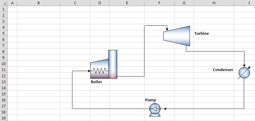
where we have a boiler, turbine (expander), condenser (cooler) and pump. Begin by creating a new blank workbook in Excel, and creating the PFD exactly as you see it above. If you wish to skip the drawing step, you may open the finished PFD from the Examples directory inside the JSteam installation directory.

Step 2 - Label the Points

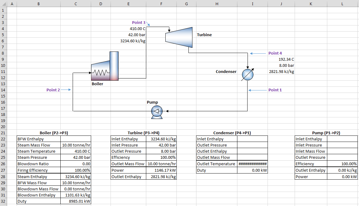
The next step is to label each point (in this case, each stream) in our PFD, so we can use them later to draw within our cycle:

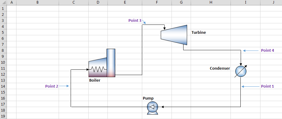
While the actual numbers don't matter, the above is a typical convention. Keep the labels in the same cells shown as we will be referencing cells later.

The points labelled above represent:

• Point 1 - Pump Input (Condenser Output)
• Point 2 - Boiler Input (Pump Output)
• Point 3 - Turbine Input (Boiler Output)
• Point 4 - Condenser Input (Turbine Output)

Whether you take an input or output centric view does not matter, as long as you are consistent. We will primarily be using these points to describe the following processes:

• P1->P2 - Represents the pump process, which takes liquid water and pressurizes it. The pump requires work to pressurize the water, which we will call wPump.
• P2->P3 - Represents the boiler process, which takes liquid water (boiler feed water) and boils it to superheated steam. The boiler requires energy to boil water, which we will call qBoiler.
• P3->P4 - Represents the turbine process, which takes superheated steam and expands it through a turbine to generate work, as well as returning superheated (just, typically) steam. The work we will call wTurbine.
• P4->P1 - Represents the condenser process, which takes the superheater steam and condenses it to liquid water (often close to saturated liquid), using cooling towers or fans. The condenser extracts energy, which we will call qCondenser.
  

Step 3 - Insert JSteam Unit Operations

As we are using JSteam, we will leverage the built in unit operations to calculate the mass and energy balances across each process. You can however perform this task using equations you may have learned in a thermodynamics class and you should return the same results.

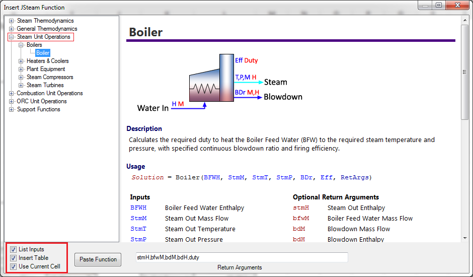
Each unit operation should be inserted using the JSteam Function Assistant from the JSteam Ribbon:

And selecting it from under the corresponding menu item on the left. Ensure all three checkboxes are ticked in the bottom left (List Inputs, Insert Table & Use Current Cell - Assuming you want to paste in the current cell!) and we will keep the default return arguments for now.

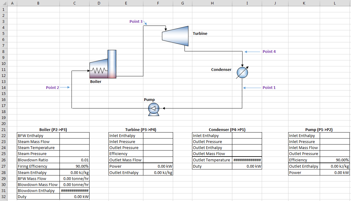
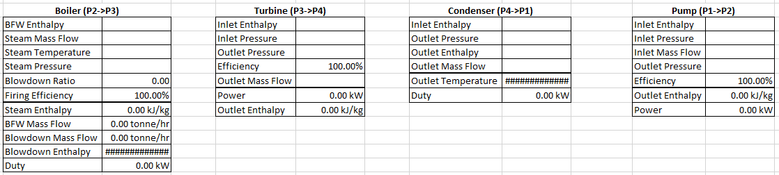
As per the below picture, insert the following four unit operations:

• Cell B22 - Boiler
• Cell E22 - Turbine1M
• Cell H22 - CoolerHM
• Cell K22 - Pump

You may wish to label each table as shown below.

Step 4 - Enter Unit Operation Default Values

Within this tutorial we will be assuming an Ideal Rankine Cycle - i.e. one where all operations are 100% efficient, there are no heating losses and pressures drops are neglected. Of course you can add these in later, but we will keep it simple for now.

Modify the following cells, as shown below:

• Boiler Blowdown Ratio - 0 (no blowdown)
• Boiler Firing Efficiency - 100%
• Turbine Efficiency - 100%
• Pump Efficiency - 100%

Step 5 - Enter Boiler Specifications

Enter the following specifications into the Boiler, as shown below:

• Steam Mass Flow - 10 tonne/hr
• Steam Temperature - 410 C
• Steam Pressure: 42 bar

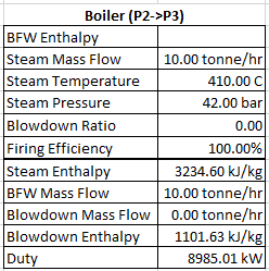
Even though we haven't filled in the Boiler Feed Water (BFW) Enthalpy, the unit solves assuming this value is 0. We now have the temperature, pressure and (specific) enthalpy values for Point 3 which we can reference to our PFD. In Cell E4 reference (using an "=") Cell C24 (Boiler Steam Temperature) to automatically link the steam temperature to Point 3 on our PFD. Cell referencing is a critical part of modelling within Excel - You should never have the same specification in more than one cell. If you need that value somewhere else, reference it.

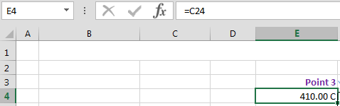
Complete the information under Point 3 by adding pressure and enthalpy too from Steam Pressure (=C25) and Steam Enthalpy (=C28), as below:

Using this technique, we can easily inspect the properties of our thermodynamic cycle before and after each process.

Step 6 - Enter Turbine Specifications

Enter the following specifications into the Turbine, as shown below:

• Inlet Enthalpy - Reference to Cell C28 (Boiler Steam Enthalpy)
• Inlet Pressure - Reference to Cell C25 (Boiler Steam Pressure)
• Outlet Pressure - 8 bar
• Outlet Mass Flow - Reference to Cell C23 (Boiler Steam Mass Flow)

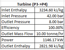
As in the previous step, we now have information we can link to a point on our PFD (Point 4), so reference the Turbine outlet pressure and enthalpy to Cells J10 and J11 respectively, and calculate the temperature using TPH(J10,J11) in Cell J9:

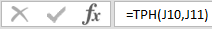
You may need to add the temperature Style by clicking on Cell J9, then clicking on the JSteam Ribbon -> Style -> Temperature. Your PFD should now look the same as below:

Step 7 - Enter Condenser Specifications

For the condenser we have chosen to use the HM (Enthalpy + Mass Flow) model, as opposed to the other varieties. It is always preferable to use enthalpy rather than temperature, as it better defines the saturated region. In this case we will specify the condenser to output saturated liquid, which if specified using the TM model, would default to saturated vapour.

Enter the following specifications into the Condenser, as shown below:

• Inlet Enthalpy - Reference to Cell F28 (Turbine Outlet Enthalpy)
• Outlet Pressure - Reference to Cell F24 (Turbine Outlet Pressure)
• Outlet Enthalpy - Insert HPX(I23,0) to calculate the enthalpy of saturated liquid (X = 0) at the unit's specified outlet pressure.
• Outlet Mass Flow - Reference to Cell F26 (Turbine Outlet Mass Flow)

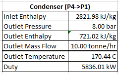
Then formula for Cell I24 (Outlet Enthalpy) is shown below:

Noting our condenser is cooling the input steam to saturated liquid only, rather than subcooling it. This is unusual in practice, as saturated liquid can cause cavitation within the pump, but it keeps things simple here. Alternatively you could use the TM cooler model and specify a temperature less than the saturated temperature for the operating pressure.

As per the previous step, we can now reference the data to a point on our PFD (Point 1), so reference the Outlet Pressure and Outlet Enthalpy to Cells J16 and J17 respectively, and calculate the temperature using TPH(J16,J17) in Cell J15.

Step 8 - Enter Pump Specifications

Enter the following specifications into the Pump, as shown below:

• Inlet Enthalpy - Reference to Cell I24 (Condenser Outlet Enthalpy)
• Inlet Pressure - Reference to Cell I23 (Condenser Outlet Pressure)
• Inlet Mass Flow - Reference to Cell I25 (Condenser Outlet Mass Flow)
• Outlet Pressure - Reference to Cell C25 (Boiler Steam Pressure)

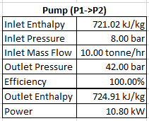
As per the previous step, link the outlet pressure and enthalpy to Cells B16 and B17 respectively, and calculate the temperature using TPH(B16,B17) in B15.

Step 9 - Complete Energy Balance

Now that we have calculate the enthalpy of the boiler feed water (the outlet enthalpy of the pump), we can connect input it to the Boiler. In the BFW Enthalpy reference Cell L27 (=L27) to complete the energy balance. Your PFD should look like the below:

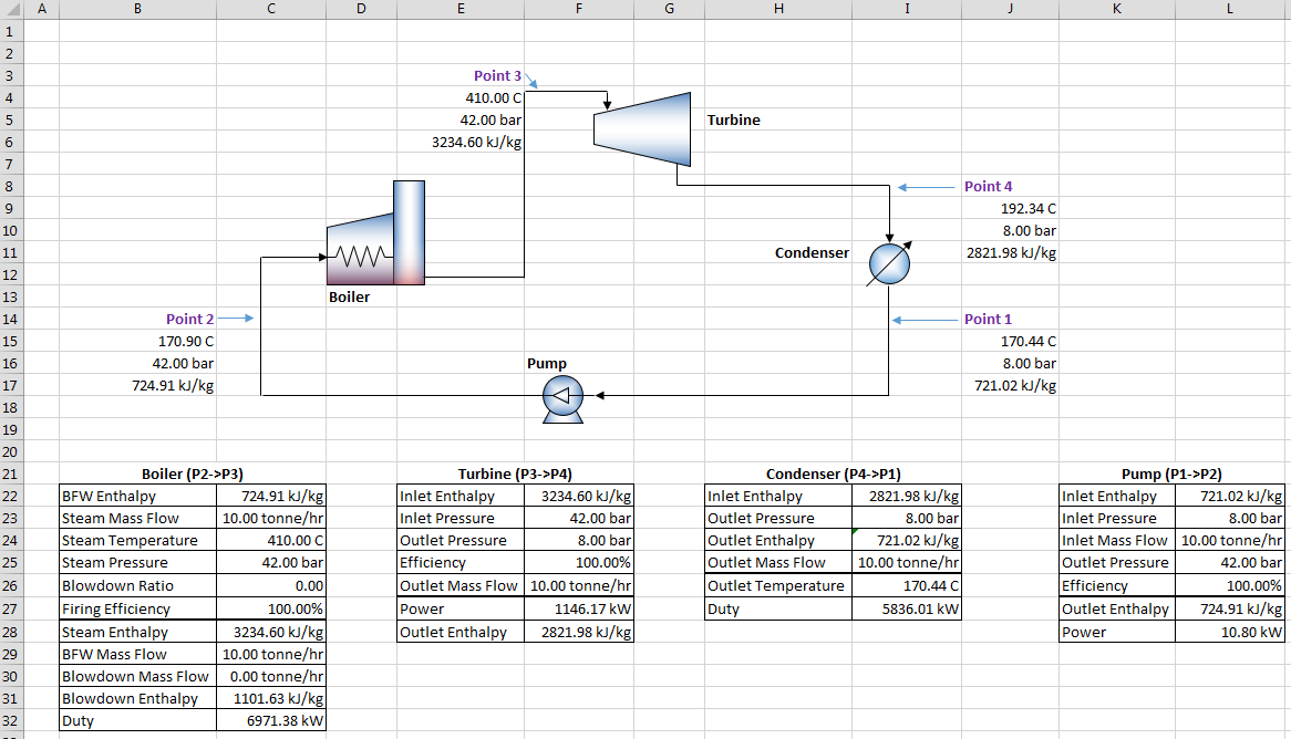
Step 10 - Check Energy Balance

Whenever modelling you should always perform a number of sanity checks. For this model, the best sanity check is an energy balance across all four operations. We know the total energy/work in must equal the total energy/work out, so let us check it:

Enter the following formula into Cell L6:

Which is equivalent to Boiler Duty + Pump Work - Condenser Duty - Turbine Work (as per the first equation). All going to plan this should result in zero:

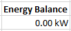
Indicating our system has been modelled correctly (you may need to paste the Power Style to see it in kW). Note this balance will not hold using the above equation if the boiler efficiency is changed or other loss is unaccounted for.

Step 11 - Calculate Thermal Efficiency

Another common calculation is that of the thermal efficiency of a Rankine cycle. There are multiple ways this can be accomplised, with various approximations, however the two below are accurate for our purposes:

or

Enter the above equations into Cells L9 and L10 (you can work out which cells need to be referenced) and you should obtain the same results as below:

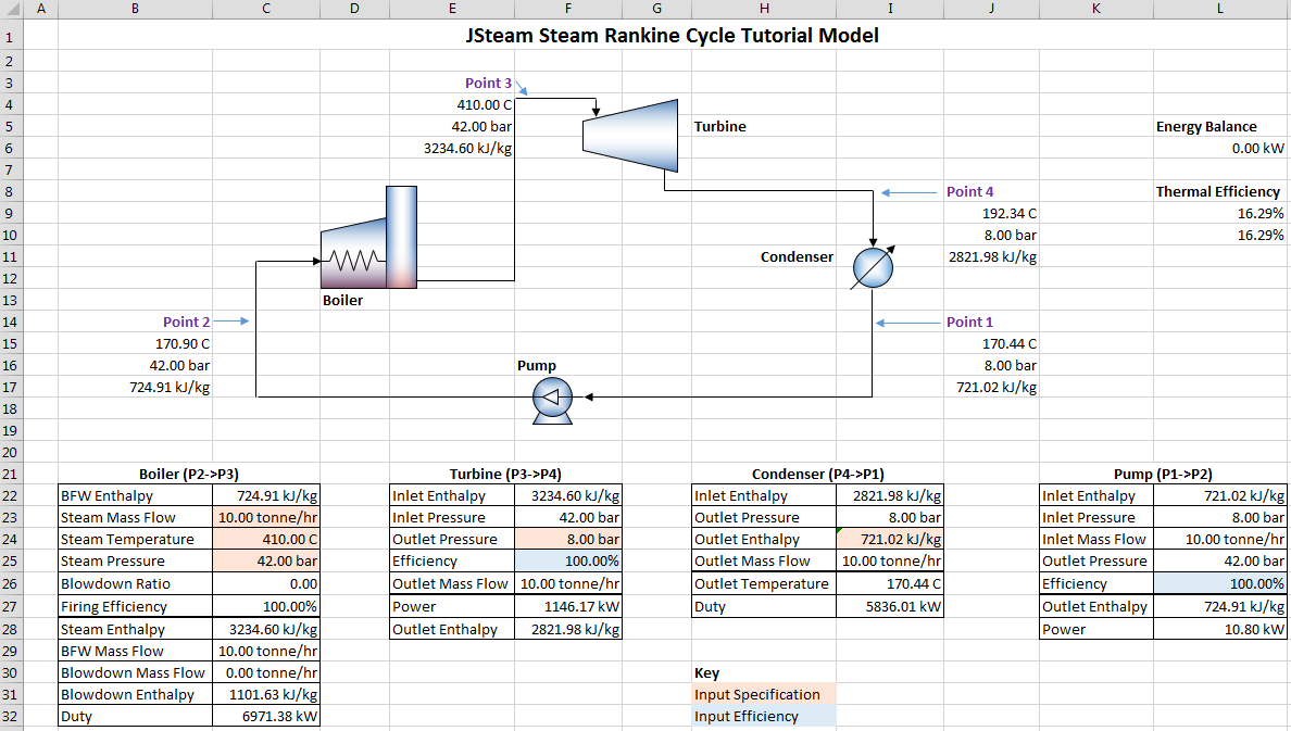
Note in the above PFD I have highlighted the cells which contain input specifications. This is good practice so you can easily find where to change specifications when moving the operating point later on.

Step 12 - Draw the TS Diagram

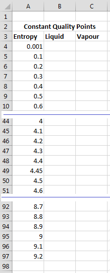
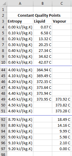
Within the same Excel Workbook, but on a different Excel Sheet, we will draw a TS diagram and overlay our Rankine Cycle on it. On the new sheet we will enter the range of Entropy we wish to draw our TS diagram over. For Water/Steam, we will use the following Entropy series:

0.001, 0.1, 0.2, 0.3, ..., 4.4, 4.45, 4.5, 4.6, 4.7, ...,9.2

Noting most points are spaced 0.1 kJ/(kg.K) apart, while extra points close to 0 and the critical point have been added to create a better plot. The diagram below shows how the points can be entered into Excel, noting the blue lines indicate a break in the table used for brevity. You may like to paste the Entropy style over all Entropy values.

Next we need to calculate the saturated liquid and vapour lines for our TS diagram. In the liquid column between (and including) the Entropy values of 0.001 -> 4.45 kJ/(kg.K) add the following function:

where A4 reflects which row the formula is in (i.e. the next cell down would be A5, then A6, etc). In the Vapour column between (and including) the Entropy values of 4.45 -> 9.2 kJ/(kg.K) add the following function:

where as above, A49 reflects which row the formula is in. Paste the temperature style into the liquid and vapour columns, and your table should look like the below:

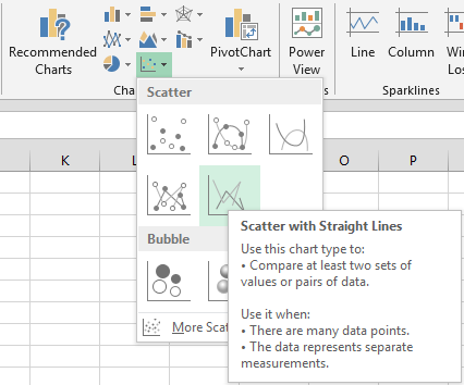
To draw the TS Diagram from the above data, assuming you have placed your table in the same cells as the picture above, select Cells A3:C97 and under the Excel Insert Tab, select Scatter, then select Scatter with Straight Lines, as shown below:

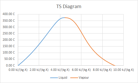
The result should be a TS Diagram for Water and Steam inserted onto your Excel Sheet, as shown below:

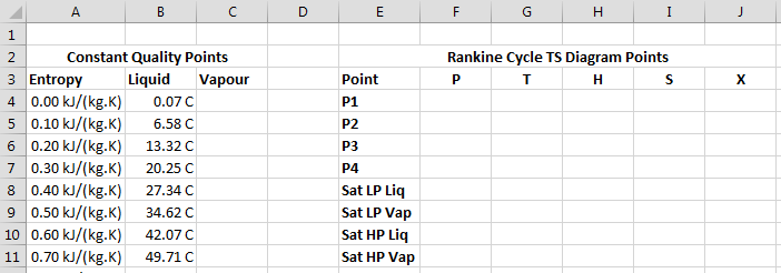
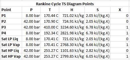
Step 13 - Construct Rankine Cycle Table

To overlay our Rankine cycle onto the TS diagram we will create a table so it is easy to select the points for plotting. Begin by setting out a table as shown below:

For points P1, P2, P3 and P4, you can reference the P, T and H values directly from the PFD, for example in P1 P (Pressure):

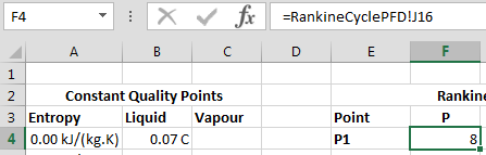
Noting to reference another sheet, simply click on the corresponding Sheet tab at the bottom of Excel, then click on the cell you want to reference. Reference the remainder of the P, T and H values for P1->P4, until you have the table below:

Complete the Entropy (S) and Quality columns for Points P1->P4 using SPH and XPH, as shown below:

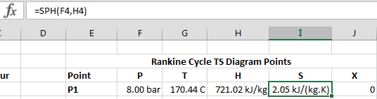
Noting we can reference the pressure and enthalpy from the current table. As mentioned above, we use enthalpy in preference over temperature (i.e. avoid SPT) for points that are close to saturation.

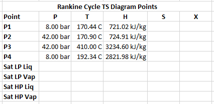
Next we will calculate the saturated liquid and vapour points for each of the pressures in the system. To begin, each Sat LP row P should be referenced to a corresponding LP pressure (e.g. Cell F4), and each Sat HP row P referenced to a HP pressure (e.g. Cell F5). For the temperature column, use TsatP to calculate the saturation temperature for the respective pressure in that row. Your table should now look like the below:

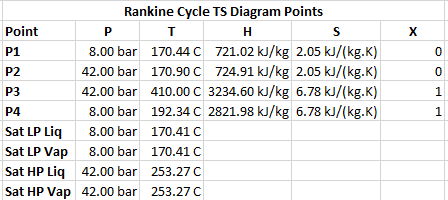
For the Quality column enter 0 for the liquid rows, and 1 for the vapour rows. In the enthalpy and Entropy Columns, use HPX and SPX respectively, referencing the row's P and X values for the arguments to the function. The final table should look like the below:

Step 14 - Add Rankine Cycle Points to TS Diagram

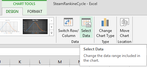
The final step in drawing the TS Diagram is to add the points in the above table to our diagram. This part is a little tedious, but only four more entries are required. Click on your Chart from Step 12, then on the Excel Ribbon Click on Chart Tools -> Design and click on the Select Data button:

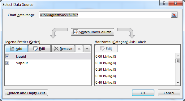
Within the Select Data Source Window, click on Add under Legend Entries:

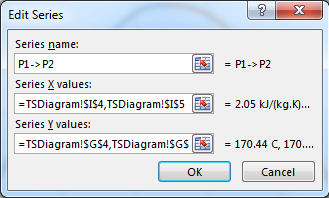
Within the Edit Series Window, enter the Series Name, X values and Y values as below (assuming your table is in the same location as this tutorial):

• Name - P1->P2
• X Values - Select Cells I4, I5
• Y Values - Select Cells G4, G5

The resulting window should look like the below:

Click OK, then repeat adding the following series for the other three processes:

• Name - P2->P3
• X Values - Select Cells I5, I10, I11, I6
• Y Values - Select Cells G5, G10, G11, G6

• Name - P3->P4
• X Values - Select Cells I6, I7
• Y Values - Select Cells G6, G7

• Name - P4->P1
• X Values - Select Cells I7, I9, I8, I4
• Y Values - Select Cells G7, G9, G8, G4

Your final TS Diagram should now look like the below:

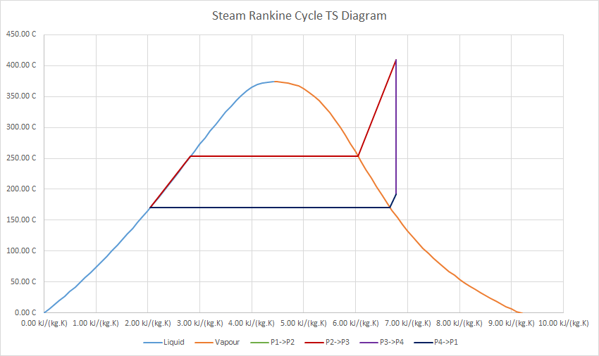
You may choose to change the colours, as I have in the above diagram. Also note that the pump process is barely visible on a TS diagram, which is typical.

Remember the above diagram is an approximation. The boiler and condenser lines should follow constant pressure lines, rather than straight line segments such as those approximated here. For information on drawing the constant pressure lines on a TS Diagram, see the TS Diagram example in the JSteam Examples folder.

Step 15 - Experiment with Non-Ideal Systems

Now that we have a model of an ideal steam Rankine cycle, we can experiment with non-ideal equipment to see the affects that real plant equipment have on the Rankine cycle. For example, try reducing the turbine efficiency to 60% (a standard number for small back pressure turbines) and examine the effect on the TS Diagram and thermal efficiency:

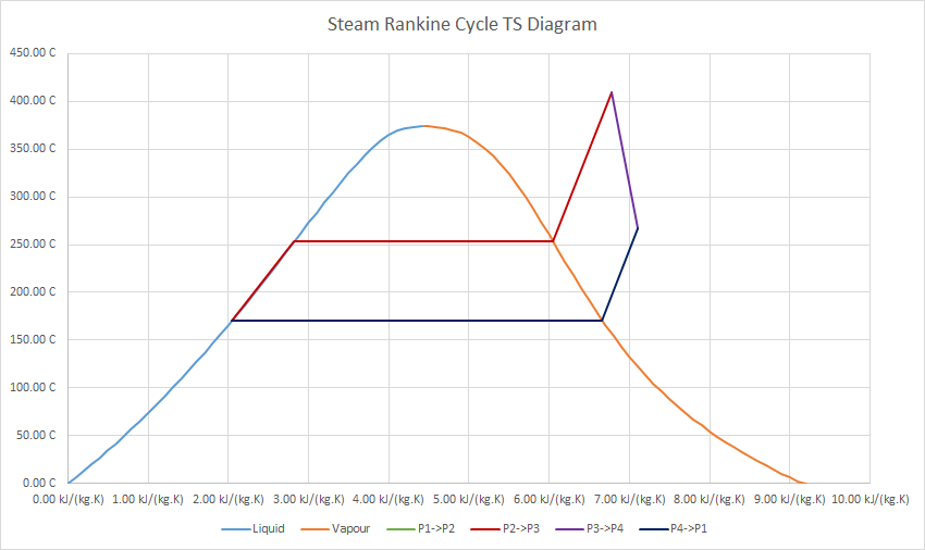
We see not only a drastic reduction in thermal efficiency, but also note the change in shape of the TS Diagram cycle - the turbine process is no longer vertical. This shows a non-isentropic process (not constant entropy) which is typical of real plant equipment.

Experiment with the model and try determine which specifications have the greatest effect on the thermal efficiency. Ensure you keep the turbine output (Point 4) as pure vapour (it is not a condensing turbine!). Hint: The current turbine outlet pressure seems quite high...

Copyright © Control Engineering