Mixture Thermodynamics
As detailed on the Nomenclature page, JSteam uses the REFPROP thermodynamic and transport property reference if a component/fluid/mixture is specified. In addition, the reader is referred to the Pure Fluid Thermodynamics Wiki page first before reading this page.
Natural Gas vs Refrigerants
JSteam provides functionality for combustion of natural gas and the calculation of the resulting combustion products, as well as organic rankine cycles where one or more refrigerants may be used as the working fluid. While the list of fluids includes fluids for both types of systems, they cannot be intermixed within JSteam. For example, it is not possible to compute the Enthalpy of a mixture of Methane and R134A, nor use it in any unit operation.
Creating Mixtures
Small (i.e. binary, ternary) Mixtures may be specified as a cell array using the following notation:
or they may be specified using the following notation, which may be easier for larger mixtures:
moleFracs = [0.5;0.5];
gasMix2 = [fluids(:),num2cell(moleFracs(:))];
In either case, the result is a cell array of fluid names and fractions which can be interpreted by the JSteamMEX interface:
2×2 cell array
{'nButane' } {[0.5]}
{'nPentane'} {[0.5]}
Fractions are always automatically normalized to 1.0 within JSteam.
Note: Fractions are always specified as mole fractions when using JSteam Toolbox and creating mixtures, and always returned from JSteam Toolbox as mole fraction specified mixtures. This is independent of the basis setting in the units setup.
Converting between Mass and Mole Fractions
If you normally work in mass fractions, you will need to convert between mass and mole fractions when using JSteam Toolbox. The interface comes with functionality to do this:
gasMixMoleFrac = {'nButane',0.5;'nPentane',0.5}
% Compute Mass Fractions
gasMixMassFrac = JSteamMEX('mole2mass',gasMixMoleFrac)
% Back to Mole Fractions (just to check)
gasMixMoleFrac_check = JSteamMEX('mass2mole',gasMixMassFrac)
Thermodynamic Property Functions
The below are some example thermodynamic routines that can be called. Note use JSteamMEX('help') to see a full list of all available property pairings for mixtures.
H = JSteamMEX('HmPT',gasMix,10,100) % Specific Enthalpy
S = JSteamMEX('SmPT',gasMix,10,100) % Specific Entropy
Cp = JSteamMEX('CpmPT',gasMix,10,100) % Isobaric Heat Capacity
Cv = JSteamMEX('CvmPT',gasMix,10,100) % Isochoric Heat Capacity
V = JSteamMEX('VmPT',gasMix,10,100) % Specific Volume
Saturation Functions
A dedicated set of functions exist for working with saturated properties of a mixture. For example, to compute the vapour pressure curve:
JSteamMEX('SetUnit','Temperature','C')
JSteamMEX('SetUnit','Pressure','kPa')
% Compute Vapour Pressure (Saturated Pressure) from -50C to Critical Temp
gasMix = {'nButane',0.5;'nPentane',0.5};
[Tc,Pc,Vc,TTrip] = JSteamMEX('Info',gasMix) % <- Important! Generates Splines for Mixture
t = linspace(-50,Tc,100);
Psat = JSteamMEX('PSatmT',gasMix,t)
% Plot a nice curve
plot(t,Psat,'.-'); grid on;
xlabel('T_{sat} [^{\circ}C]')
ylabel('P_{sat} [kPa]')
title('Vapour-Liquid Saturation Curve of 50/50 nButane/nPentane Mixture')
% Return to default units
JSteamMEX('SetDefaultUnits')

There are a range of other mixture saturation functions available from JSteam + REFPROP and the user is encouraged to use JSteamMEX('help') to identify routines as required. As per the above code snippet, requesting "Info" on a mixture before calling any saturation functions is strongly encouraged as internally REFPROP will generate splines to speed up computation. Don't call this function if you want to skip the spline interpolation.
Transport Functions
In addition to thermodynamic functions, the database also provides two routines for transport functions (thermal conductivity and viscosity). Unlike with IAPWS IF-97, REFPROP provides a large number of property pairings for computation of these properties.
K = JSteamMEX('KmPT',gasMix,10,100) % Thermal Conductivity of Mixture [mW/(m.K)]
U = JSteamMEX('UmPT',gasMix,10,100) % Viscosity of Mixture [uPa.s]
Note the default JSteam units for these properties are non-standard, but have been chosen to provide "sensible" numbers to common operating regions, and thus avoiding large numbers of decimal places.
Other Properties
In addition to the above functions, JSteam provides methods for heating value and molecular weight:
NHV = JSteamMEX('NHV',gasMix) % Net (Lower) Heating Value
GHV = JSteamMEX('GHV',gasMix) % Gross (Higher) Heating Value
MW = JSteamMEX('MW',gasMix) % Molecular Weight
as well as information on the mixture itself, and range of validity for calculations:
% Temperature of the Triple Point (TTrip)
% Normal Boiling Temperature (TNBpt)
% Acentric Factor (w)
% Temperature Validity Range (Tmin -> TMax)
% Maximum Valid Density (DMax)
% Maximum Valid Pressure (PMax)
[Tc,Pc,Vc,TTrip,TNBpt,w,TMax,TMin,DMax,PMax] = JSteamMEX('Info',gasMix)
Example: Humid Air Psychrometrics Chart
The example below shows how to create an approximate Psychrometrics chart for Humid Air. It is approximate because JSteam does not include all gases present in air (such as Argon) as well as because it approximates terms like the enhancement factor as a constant. The example is derived from this paper, and complete code found in Examples/JSteam_Psychrometrics.m.
Pamb = JSteamMEX('OneAtm'); %bar
Tamb = linspace(5,60); %C
RelHum = 0:10:100; % percent
% Constants
f = 1.0045; %enhancement factor (at approx 1 atm, 25C)
B = 0.6219907; %ratio of molecular weight
% Calculation Loop
nh = length(RelHum); nt = length(Tamb);
w = zeros(nt,nh);
for i = 1:nh
for j = 1:nt
% Saturated Water Vapour Pressure
Pws = JSteamMEX('PsatcT','Water',Tamb(j));
% Mole Fraction of Water
Xw = RelHum(i)/100*f*Pws/Pamb;
% Humidity Ratio
w(j,i) = B * Xw/(1-Xw); %[kg/kg]
end
end
% Plot
plot(Tamb,w*1e3,'color',[0 0.447 0.7410]); axis('tight');
ylim([0 30]); grid on;
xlabel('Dry Bulb Temperature [^\circC]');
ylabel('Humidity Ratio [g_w/kg_a]');
title(sprintf('Psychrometric Chart for Pressure = %g bar',Pamb));
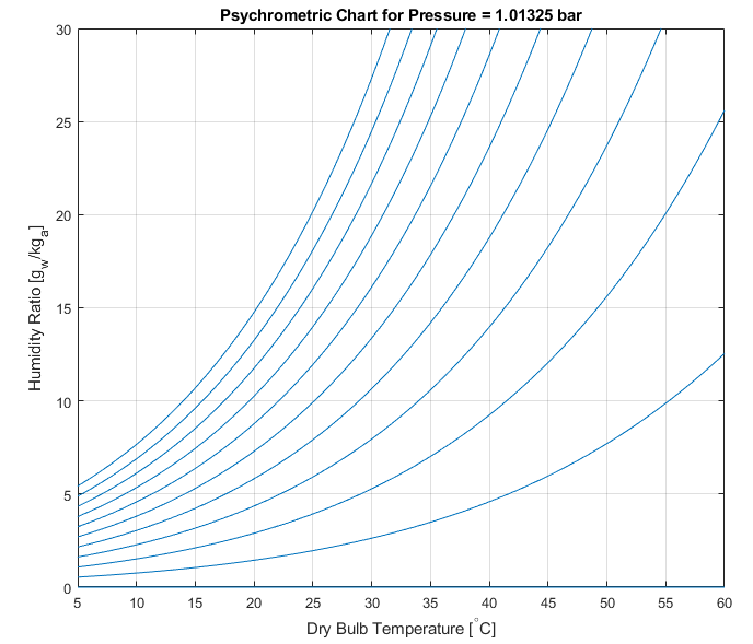
The above plot contains lines showing the Humidity Ratio (the ratio of water vapour mass to dry air mass) at various relative humidity levels (each line is a constant relative humidity), for atmospheric pressure and the given dry bulb temperature range. The chart shows, as expected, that as the dry bulb temperature increases, a given kg of dry air (kg_a) is able to support a larger mass of water vapour (g_w), noting the differences in units.
Given Humid Air is so important for modelling utility systems, where the amount of water in the air can substantially effect the efficiency of a combustion chamber, JSteam also comes with a routine to help create a humid air mixture with a given amount of relativity humidity (fraction) at the given atmospheric conditions:
To test this routine, together while demonstrating the mole2mass functionality, the above plot is overlaid with the humidity ratio manually calculated.
Tamb = min(Tamb):5:max(Tamb); %C
% For each humidity point
for i = 1:length(RelHum)
% For each temperature point
for j = 1:length(Tamb)
% Set as Spec Above use built in JSteam Function
humAir = JSteamMEX('humidair',RelHum(i)/100,Pamb,Tamb(j));
% Manually Calculate Humidity Ratio and Compare to Psychrometric Chart
massFrac = JSteamMEX('mole2mass',humAir);
idx = strcmpi(massFrac(:,1),'Water');
if(any(idx))
fracs = [massFrac{:,2}]';
%kg water / kg of air
wman = sum(fracs(idx))/sum(fracs(~idx));
else
wman = 0;
end
% Add to our existing plot
hold on
plot(Tamb(j),wman*1e3,'r.','markersize',15)
hold off
end
end
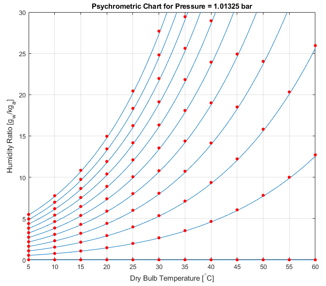
Ideally, the red dots would be exactly located on top of the blue lines, but with the missing trace gases not included in the JSteam mixture (it only models N, O, CO2, H2O), the ratio of molecular weight is not the same as the previous example. It is however good enough for most purposes.