Organic Rankine Cycle Unit Operations
In addition to suppling thermodynamic and transport routines, JSteam also provides a suite of models (known as unit operations) for modelling subsystems and equipment within heat and power plants. This page covers the Organic Rankine Cycle and Refrigerant unit operations, common in GeoThermal and other low temperature working fluid power plants. These functions rely on the MixtureThermodynamics functionality included in JSteam. These unit operations are very similar to the Steam Unit Operations thus it is highly recommended to read that section first.
To view available unit operations, use JSteamMEX('help') under the REFRIGERANT UNIT OPERATIONS heading. They are grouped as follows:
- Compressors
- Single and multi-stage compressors, with duty and mass flow variants.
- Coolers & Heaters
- Simple duty and mass flow specified heaters and coolers.
- Plant Equipment
- Other models such as valves, pumps, deaerators, and flash drums.
- Expanders/Turbines
- Single and multi-stage expanders/turbines, with duty and mass flow variants.
Example: Evaporator
This example follows the OEC-1 Miravalles Geothermal Model Tutorial at Step 4:
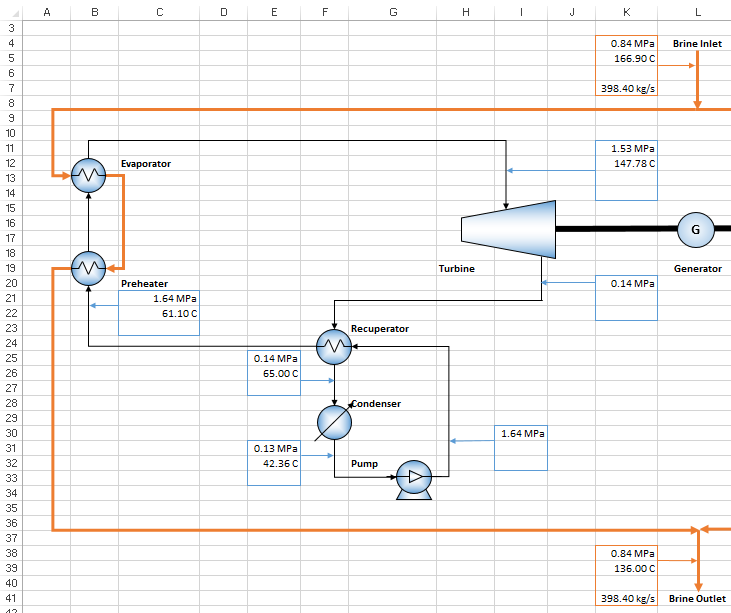
We are going to model the lumped Preheater + Evaporator as a single heat exchanger, using the same technique as done for Steam Heat Exchangers by splitting it into a heater and cooler. The full code is in Examples/JSteam_UnitOps.m:
JSteamMEX('SetUnit','Pressure','MPa');
JSteamMEX('SetUnit','MassFlow','kg/s');
% Brine Specs
brine = {'water',1}; % Assume just water
brineInP = 0.84; % Brine input pressure [MPa]
brineInT = 166.9; % Brine input temperature [C]
brineInH = JSteamMEX('HmPT',brine,brineInP,brineInT); % Inlet Enthalpy [kJ/kg]
brineInM = 398.4/2; % Brine input mass flow rate [kg/s] (50% each side)
brineOutT = 136.0; % Brine outlet temperature [C]
% Working Fluid Specs
fluid = {'nPentane',1}; % 100% n-Pentane
fluidInP = 1.64; % Fluid input pressure [MPa]
fluidInT = 61.1; % Fluid input temperature [C]
fluidInH = JSteamMEX('HmPT',fluid,fluidInP,fluidInT); % Inlet Enthalpy [kJ/kg]
fluidOutT = 147.78; % Fluid outlet temperature [C]
fluidOutP = 1.53; % Fluid outlet pressure [MPa]
% Solve Cooler (Brine, have T+M, solve H+Q):
brineOutP = brineInP; % Assume no pressure drop
brineOutM = brineInM; % Assume no mass loss
[status,brineOutH,Duty] = JSteamMEX('UnitOp_CoolerTMC',brine,brineInH,brineOutP,brineOutT,brineOutM)
% Solve Heater (Working Fluid, have T+Q, solve H+M):
[status,outH,outM] = JSteamMEX('UnitOp_HeaterTQC',fluid,fluidInH,fluidOutP,fluidOutT,Duty)
% Return to default units
JSteamMEX('SetDefaultUnits');
The above example uses the input and output measurements of the brine side of the system to solve the overall duty of the exchanger, which is then used to compute the total mass flow of the working fluid through the heater. This results in 56.58kg/s for a duty of 26537.8kW.
Note, the only difference between refrigerant and steam unit operations is the extra "C" in the end of the name, and the first argument expects a refrigerant mixture. All functionality is exactly the same, just changing what thermodynamic package is called underneath.