Water & Steam Thermodynamics
As detailed on the Nomenclature page, JSteam uses the IAPWS IF-97 thermodynamic and transport property reference if a component/fluid/mixture is not specified.
Thermodynamic Property Functions
The below are some example thermodynamic routines that can be called. Note use JSteamMEX('help') to see a full list of all available property pairings.
S = JSteamMEX('SPT',1,100) % Specific Entropy
Cp = JSteamMEX('CpPT',1,100) % Isobaric Heat Capacity
Cv = JSteamMEX('CvPT',1,100) % Isochoric Heat Capacity
V = JSteamMEX('VPT',1,100) % Specific Volume
In addition to the above "forward" functions, the reference database also includes selected "reverse" functions:
T = JSteamMEX('THS',H,S) % Temperature
Using the above reverse functions from IAPWS IF-97 you will start to see the accuracy of the database. Note if you require Water/Steam thermodynamic calculations as accurate as possible, you can use REFPROP, e.g.
S = JSteamMEX('ScPT','water',1,100) % Specific Entropy of Steam
P = JSteamMEX('PcHS','water',H,S) % Reverse Pressure
T = JSteamMEX('TcHS','water',H,S) % Reverse Temperature
which will gain a few extra decimal places of accuracy (typically), at a cost of computational speed.
Saturation Functions
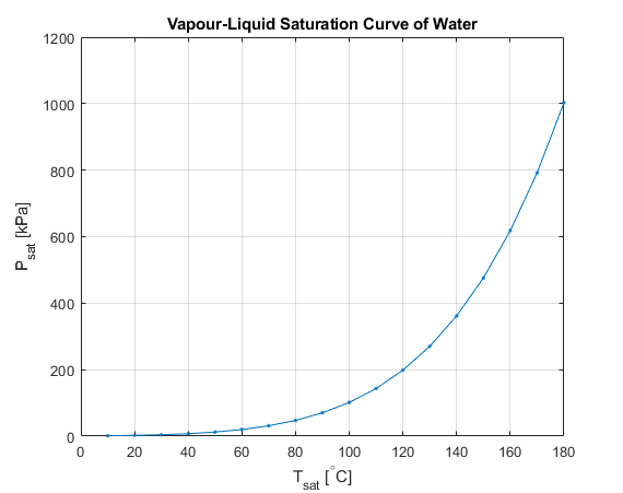
A dedicated set of functions exist for working with saturated (i.e. not sub-cooled/super-heated) properties of water. For example, to compute the vapour pressure curve:
JSteamMEX('SetUnit','Temperature','C')
JSteamMEX('SetUnit','Pressure','kPa')
% Compute Vapour Pressure (Saturated Pressure) across this temp range
t = 10:10:180;
Psat = JSteamMEX('PSatT',t)
% Plot a nice curve
plot(t,Psat,'.-'); grid on;
xlabel('T_{sat} [^{\circ}C]')
ylabel('P_{sat} [kPa]')
title('Vapour-Liquid Saturation Curve of Water')
% Return to default units
JSteamMEX('SetDefaultUnits')

Other functions exist to compute thermodynamic properties at specific saturated states. For example, to compute the Enthalpy of Vaporization of water at one atmosphere:
P = JSteamMEX('ConvUnit',1,'atm','bar'); % 1atm in bar
% Determine Enthalpy of Saturated Vapour (X=1) at 1 atm
HsatV = JSteamMEX('HPX',P,1)
X = JSteamMEX('XPH',P,HsatV) % check quality
TsatV = JSteamMEX('TPH',P,HsatV)
% Determine Enthalpy of Saturated Liquid (X=0) at 1 atm
HsatL = JSteamMEX('HPX',P,0)
X = JSteamMEX('XPH',P,HsatL) % check
TsatL = JSteamMEX('TPH',P,HsatL)
% Determine Enthalpy of Vaporization
HVap = HsatV - HsatL
% IAPWS 97 Temperature Error
tempError = TsatV-TsatL % should be 0
The above example shows the "X" functions, which include specifying a specific quality (amount of saturated liquid vs saturated vapour, between 0 -> 1), as well as computing the quality as a function of e.g. pressure and enthalpy. It also demonstrates the accuracy of the Temperature reverse functionality, where the temperature should be the same at both the saturated vapour and liquid points (which is why you can't specify a saturated state using pressure and temperature alone), but the IAPWS IF-97 database has an error of approximately 0.001 degC. The user can repeat the above exercise using REFPROP to see this error reduce to 0.
Transport Property Functions
In addition to thermodynamic functions, the database also provides two routines for transport functions (thermal conductivity and viscosity). These are only for pressure and temperature pairings, as below:
U = JSteamMEX('UPT',1,100) % Viscosity of Steam [uPa.s]
Note the default JSteam units for these properties are non-standard, but have been chosen to provide "sensible" numbers to common operating regions, and thus avoiding large numbers of decimal places.
Example: Mollier Diagram
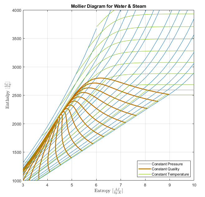
The following example shows how to generate the data to draw a Mollier (H vs S) diagram for Water & Steam:
s_range = 3:0.25:10;
p_range = [0.01 0.02 0.04 0.1 0.2 0.5 1 2 6 10 20 50 ...
100 200 500 1e3];
[S_conP,P] = meshgrid(s_range,p_range);
H_conP = JSteamMEX('HPS',P,S_conP);
% Enthalpy & Entropy at Constant Quality
x_range = 1:-0.05:0;
p_range = [0.01:0.01:0.1 0.2:0.1:1 2:1:10 20:10:220];
[X,P] = meshgrid(x_range,p_range);
H_conX = JSteamMEX('HPX',P,X);
S_conX = JSteamMEX('SPH',P,H_conX);
% Lines of Constant Temperature
t_range = [10 50 100:100:800];
s_range = 10:-0.01:3;
[T,S_conT] = meshgrid(t_range,s_range);
H_conT = JSteamMEX('HTS',T,S_conT);

The full example is in Examples/JSteam_SteamMollier.m.