JSteam

SymUtility is a MATLAB class that inherits and adds functionality from OPTI Toolbox's SymBuilder class. This allows a user to construct utility system models symbolically (i.e. an equation based model) and automatically prepare them for optimization. It also includes multiple part-load models based on industrial data which are not included in the standard JSteam model library.

The user is encouraged to read Chapter 5 and Chapter 6 of my thesis for information on the part load model derivation and range of applicability, together with how SymUtility models can be constructed and optimized in MATLAB. Using this approach, it is possible to simulate and optimize large-scale systems in fractions of a second, including to global optimality using OPTI Toolbox's White Box Optimization functionality.

A full SymUtility optimization model from my thesis is included in Examples/SymUtilityModels to demonstrate the modelling approach, including how JSteam Excel and JSteam Toolbox can be connected to easily visualize optimization results. The examples below are only to show a brief overview of the included functionality, and can be found in Examples/JSteam_SymUtility.m.

Fixed Efficiency Back Pressure Steam Turbine Model

A simple model provided by SymUtility is the fixed efficiency (i.e. the Isentropic efficiency does not vary with load) back pressure turbine model. Many systems include steam turbines that are connected to fixed mechanical loads and therefore the part-load aspect does not need to be modelled as accurately, as either the turbine runs the load, or an electric motor runs the load, depending on the economics of the utility system (i.e. where the optimization comes in!). This can be added to a SymUtility model as follows:

What the above code is doing is creating three models (note the output arguments are not required, they are included here just for explanation):

expQ:An expression for output power, as a function of input enthalpy and mass flow rate.

expH:An expression for output enthalpy, as a function of input enthalpy and mass flow rate.

conQ:A constraint which states that if the turbine is "on", that the output power must equal the rated power, as a function of input enthalpy and mass flow rate.

For example, the expression for output power, noting the symbolic variables m1 and h1:

SteamTurbine1_Q = m1*(1/3.6)*0.7*(-409.572203943965 + 0.211397887168034*h1)

The above is the standard equation for output power across an expander with a fixed Isentropic efficiency (0.7 in this case), with the thermodynamics (i.e. the Isentropic enthalpy drop across the expander) modelled as a straight line approximation, centered on the reference operating point (from the incoming specifications). This means at the reference operating point, the model is approximately "perfect", while as the input enthalpy moves further from the reference point, the accuracy will gradually degrade. This is demonstrated below:

showing almost identical results (as expected), while if the input operating point moves too far from the regression point:

the error increases. Additionally to inspect the power output constraint:

we see the constraint is invalid, as the input mass flow rate for the given turbine specifications and input enthalpy does not result in meeting the mechanical power output requirement. Note that all the regressions in expressions and constraints are automatically computed by SymUtility, and is one the reasons it makes it a powerful tool.

If you are interested in how SymUtility has saved the model (so far), you can inspect the properties of the underling SymBuilder object:

Viewable above we can see the mechanical output power constraint (view properties cl and cu to see constraint bounds), together with expressions (to be substituted into constraints or the objective later), together with variable bounds and variable types, which in this case has bST1 as a binary variable (as intended). While this is far from a complete system model, it shows how incrementally, using the functions provided with SymUtility, one could build up complex optimization models with minimal user input.

Part Load Turbo Generator Steam Turbine Model

A more complex variation of the back pressure turbine model above is a part-load turbo generator model. This model includes variable Isentropic efficiency based on the fraction of full load it is operating at, derived from industrial data for a similarly sized turbine. A turbo generator is often run at varying loads in order to meet the electricity demand of the utility system, and thus the part load behaviour of the unit must be accounted for in the model. Consider the following 200kW example:

Notice that the model does not require an efficiency input, and instead will calculate one based on looking up similar sized turbines from an internal dataset. It returns the regression parameters together with some functions which can be used to plot the turbine response across load:

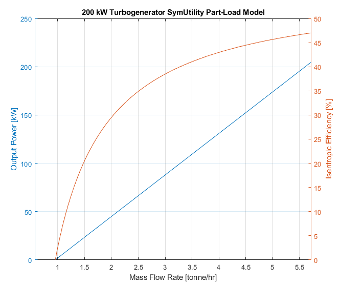
The model demonstrates that a minimum mass flow must be achieved in order to begin power generation (i.e. this model includes spinning losses which must be overcome), together with the classic "Willans Line" showing a linear relationship between mass flow rate and output power. The efficiency model shows a steep nonlinear effect between load and efficiency, which is critical to model for this unit.

The above example is not required by the user to be called, but is useful to understand what is happening "behind the scenes". The normal function call would be:

Looking at the expression for output power:

we can see the expression is bilinear (products of two variables only), while the output enthalpy expression is nonlinear due to the ratios calculated:

Both models include a binary variable with two constraints that force an "OR" condition, which enforces that if the turbo generator is "on", then it must be providing at least the minimum mass flow to ensure a positive output power, otherwise the mass flow must be 0 and the power output is forced to 0.

Part Load Fired Boiler Model

A key cost of a utility system is the fuel supply to the boiler(s), and therefore must be accurately modelled across the operating range of the boiler(s). This requires a part-load model is derived. Consider the following example:

Notice that the model accepts an operating range (steam production mass flow range) which it uses to generate the model, together with loss data from literature which is stored internally. It returns the regression parameters together with some functions which can be used to plot the boiler response across load:

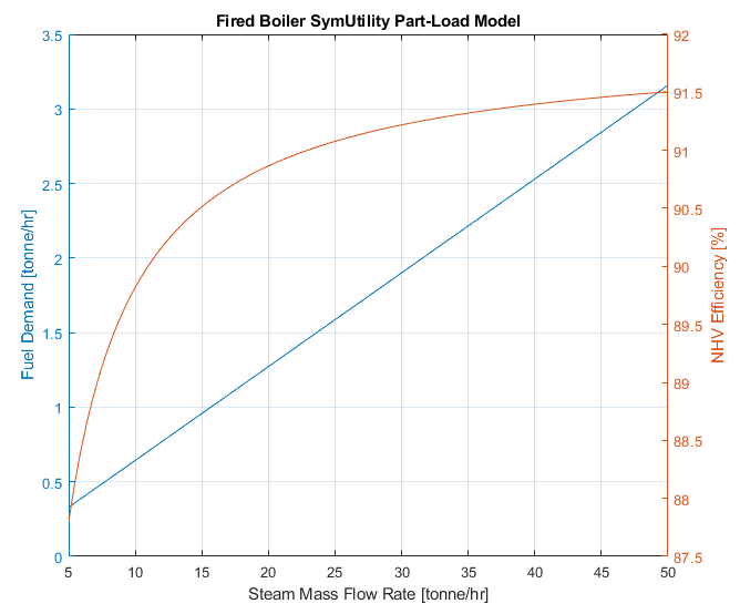
The model demonstrates a (approximately, due to the model formulation) linear relationship between steam production and fuel demand, regressed to the operating range of the boiler, the fuel in use, atmospheric conditions and industrial loss data (boiler surface, flue gas losses) for boilers. The efficiency model is also plotted for interest, but based on the modelling approach, can be linearized into the steam vs fuel expression.

The above example is not required by the user to be called, but is useful to understand what is happening "behind the scenes". The normal function call would be:

we can see the fuel mass flow expression is linear:

but includes a binary variable with two constraints that force an "OR" condition, which enforces that if the boiler is "on", then it must be providing at least the minimum mass flow, otherwise the mass flow must be 0, similar to the turbo generator model.

Constructing a SymUtility Optimization Model

So far this page has demonstrated some of the advanced models present in the SymUtility class, however its real power is being able to create full utility system models and optimize them subject to a user specified (typically economic) objective function. The below example is an open loop (i.e. no turbine output steam recovery, which is not realistic, but keeps this example simpler) utility system with a 50 tonne/hr fired boiler supplying steam into a High Pressure (HP) steam header, which then feeds a 1MW steam turbo generator and a 500kW back pressure turbine connected to a 500kW mechanical load. The objective is to minimize the cost of running the utility system, while still providing (at a minimum) the 500kW mechanical load demand. Options the optimizer could find include:

1. Don't produce any steam, and simply buy electricity to run the 500kW load.
2. Produce enough steam to run the back pressure turbine, but don't run the turbo generator.
3. Produce enough steam to generate 500kW from the turbo generator to run the 500kW mechanical load, but don't sell excess power. Don't run the back pressure turbine.
4. Produce enough steam to generate the full 1MW from the turbo generator, use 500kW for the mechanical load, and sell the excess power. Don't run the back pressure turbine.
5. +Others!

It is critical when optimizing these systems to hypothesize the results you expect, in order to sanity check what the optimizer has returned. When modelling systems you should always start with a PFD and name the mass flow and enthalpy variables across the system, such as done in Examples/SymUtilityModels/Aguilar3HDR.png. Because this system is so simple, we can just list the variable names here:

To begin, we load SymUtility and begin entering the mass and energy balance equations of the system:

Next, we add the unit operation models and their specifications:

the next step is to tell the optimizer what our objective is. To do this we need to enter the costs of fuel gas (FG, for the boiler), as well as the cost of buying electricity (BElec) and the price of selling electricity (SElec), together with forming the overall power balance of the system:

The power balance function adds a binary variable that allows us to determine in the objective function whether we are buying (bp=1) or selling (bp=0) electricity. The objective then is simply how much it costs in fuel gas and electricity to run the system. We then call Build on the final SymUtility object to construct our optimization problem!

As shown above, it took less than half a second to generate the optimization problem, including first and second derivatives, and determine the type of problem we are solving. In this case it is a MINLP as it contains a nonlinear objective and binary variables.

In order to optimize the resulting model, we will need to supply the optimizer with an initial starting guess. To know what variables the optimizer has placed in which order in the decision variable vector, use:

From above we can see the binary variables are first, followed by the HP Header enthalpy, and then the 5 mass flow variables. Note enthalpy variable H1 has been symbolically eliminated (it was redundant), but we used in our modelling approach to keep the equations easier to understand.

Typically you should provide the best estimate possible for the optimizer in order to obtain a true optimum (or even, allow the optimizer to find a solution). This can be done by using guesses from an associated JSteam Excel model of the system, or a JSteam Toolbox model built in MATLAB. For this problem, given it is so small, we will just use all zeros, but note this will not work for real systems!

Using the Results method allows an easy to view console output of the operating point solved:

From the above print out we can see the optimized operating point was found in 0.11s, and the operating point found was Case (2), with the back pressure turbine fed by the boiler, and the turbo generator not running.

At this point we can explore the other results we could expect the optimized model to solve. For example, increasing the fuel cost should result in the optimizer choosing to buy electricity and shut down steam production:

Or we could model a spike in electricity sell price (i.e. the electricity network requires more generation) so that the turbo generator is enabled and 1MW is exported:

The above example is just a toy problem for ease of demonstration, however the reader is referred to Examples/SymUtilityModels in the toolbox for a full 3-Header Steam Utility system with example Excel Interface PFD, Sequential Simulation Model and SimUtility Optimization Model.