Basic OPTI Usage
Welcome to the OPTI getting started tutorial! This page will aim to teach you enough to start building and solving optimization problems. This tutorial assumes you have downloaded and installed OPTI by running opti_Install.m.
Creating an Optimization Interface (OPTI) Problem
Creating an OPTI problem requires using the OPTI class, a simple MATLAB class which handles the interfacing (and conversions) between your problem and the desired solver.
To create an OPTI object, you name and pass the arguments to the OPTI constructor in the following manner:
In the above example fun is a function handle to a standard MATLAB function containing a nonlinear objective, lb and ub are upper and lower bounds on the decision variable x, and x0 is the initial guess of our problem. Using the supplied arguments OPTI will automatically determine we are solving a constrained nonlinear program (NLP) and set up the problem to be solved by the best NLP solver available.
Note best refers to my choice of best, and you are encouraged to try other solvers to see which works best for your problem! We will see changing options and solvers shortly.
You will note all arguments are proceeded by a string, indicating to OPTI what the argument contains. You can also group arguments, such as done with 'bounds' to supply both upper and lower bounds. To find all fields available simply type:
which will list and describe all fields and groups availables.
Example 1: Small LP
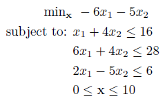
The above problem is an example of a small linear program, a common starting point when learning optimization! The problem can be entered into OPTI as follows:
f = -[6 5]'; %Objective Function (min f'x)
A = [1,4; 6,4; 2, -5]; %Linear Inequality Constraints (Ax <= b)
b = [16;28;6];
lb = [0;0]; %Bounds on x (lb <= x <= ub)
ub = [10;10];
% Create OPTI Object
Opt = opti('f',f,'ineq',A,b,'bounds',lb,ub)
To solve the problem simply call the solve method:
Providing your problem is feasible (and the solver can find a solution) x will contain the solution vector, fval the objective value at the solution, exitflag the solver exit status and info a structure with solver run information.
Common exit flags include:
Alternative Setup Strategies
To accommodate users with different nomenclature or preferences, the OPTI object created in the above example could also be created as follows:
% OR
Opt = opti('grad',f,'ineq',A,b,'bounds',lb,ub); %grad = f
% OR
Opt = opti('f',f,'A',A,'b',b,'bounds',lb,ub); %individual A,b
% OR
Opt = opti('f',f,'ineq',A,b,'lb',lb,'ub',ub); %individual lb,ub
It is important to note two things at this stage: a) the same argument can have multiple names (e.g. c, f and grad all refer to a linear objective, you choose the name most meaningful to you), as well as b) grouping of arguments is optional.
Choosing a Solver
So far OPTI has chosen the solver it has determined as the best for the problem entered. You may choose, however, to customize the solver choice. To start with, we need to determine which solvers are available on your system:
The above function will list all solvers and their versions installed on your system. However, more interesting is determining what solvers solve what problem types! You can generate a problem vs solver matrix by typing:
You can also determine the available solvers by a specific problem type by passing the problem type as a string. For example to display all installed solvers which can solve Linear Programs (LP) type:
The above method will also display compatible constraint types of each solver (e.g. an NLP solver may use linear inequalities but not nonlinear inequalities). To display all information about a solver and its interface, using the following code (for e.g. CLP):
To supply the solver choice to OPTI, it is passed via a dedicated options interface. This not only allows the solver to be specified but also many other options such as maximum iterations, maximum time, convergence tolerances and so forth. You can view all common options by typing:
optiset will generate an options structure compatible with opti, with defaults set to values you did not specify. Getting back to our solver specification with our LP, this can be achieved as follows:
opts = optiset('solver','clp');
%Rebuild the problem passing the options via the 'options' argument
Opt = opti('f',f,'ineq',A,b,'bounds',lb,ub,'options',opts)
Common Options
Once you are suitably familiar with your solver it is likely you will want to customize the way it behaves. To see what options are available for your solver you can type:
which will generate a solver vs option matrix. Note the option names are abbreviated for display reasons, however I'm sure you can match them to those in optiset!
Three common options I use are display set to iter to display iteration by iteration solver progress, maxiter set to the maximum iterations for the solver to run and maxtime to limit the maximum execution time of the solver. Note not all solvers support all options, so check the solver vs option table to see what is supported.
Example 2: Rosenbrock NLP
The Rosenbrock 'banana' function is a classic nonlinear optimization test problem:
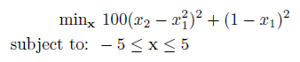
Note the original Rosenbrock function is unconstrained, and I have artificially added bounds to the problem. This is generally a good idea as it will help the solver scale the problem, as well as reduce the search space.
The problem can be created and solved as follows:
fun = @(x) 100*(x(2) - x(1)^2)^2 + (1 - x(1))^2;
% Constraints
lb = [-5;-5];
ub = [5;5];
% Initial Starting Guess (Required for Nonlinear Problems)
x0 = [0;0];
% Setup Options
opts = optiset('solver','lbfgsb','display','iter');
% Create OPTI Object
Opt = opti('fun',fun,'bounds',lb,ub,'options',opts)
% Solve!
[x,fval,ef,info] = solve(Opt,x0)
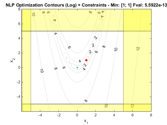
With one and two variable problems we have the luxury of being able to plot the problem (OPTI v2.00 can plot higher dimensional problem as well). With OPTI this can be achieved directly from the OPTI object:
Summary
This brief summary concludes your introduction to OPTI. There are plenty more examples so continue to browse, or better yet, jump in and have a go for yourself. If you are familiar with the MATLAB Optimization Toolbox you may like to begin by having a look at the OPTI overloads.