Two Ways to Define Constraints
OPTI allows both standard ways of specifying inequality and equality constraints when creating an optimization problem. The first method is when inequality and equality constraints are treated separately, and the second when row constraints are used.
As the format varies between the linear and nonlinear case, we will address each below.
Linear Constraints
Linear constraints can be entered in one of two forms:

The general MATLAB format is specifying individual matrices and vectors for inequalities and equalities. An example definition is shown below:
However a more efficient method is specifying all linear constraints via one matrix, A and two vectors, rl and ru. The advantage is being able to specify two inequalities for each row of A, if required. An example is shown below:
To specify an equality constraint using the above row method, simply specify the corresponding element in both rl and ru to the equality value.
Example 1: Linear Constraints with an LP
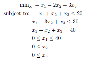
Consider the following problem from the LP examples section:

To begin, we will enter it in MATLAB format (separate inequalities and equalities):
f = -[1 2 3]';
% Inequality Constraints (Ax <= b)
A = [-1 1 1;
1 -3 1];
b = [20;30];
% Equality Constraints (Aeqx = beq)
Aeq = [1 1 1];
beq = 40;
% Bounds (lb <= x <= ub)
lb = [0;0;0];
ub = [40;Inf;Inf];
% Build OPTI Object
Opt = opti('f',f,'ineq',A,b,'eq',Aeq,beq,'bounds',lb,ub)
% Solve Problem
[x,fval] = solve(Opt)
Now lets repeat, this time entering it in row format:
f = -[1 2 3]';
% Row Constraints (rl <= A*x <= ru)
A = [-1 1 1;
1 -3 1;
1 1 1];
rl = [-Inf;-Inf;40];
ru = [20;30;40];
% Bounds (lb <= x <= ub)
lb = [0;0;0];
ub = [40;Inf;Inf];
% Build OPTI Object
Opt = opti('f',f,'lin',A,rl,ru,'bounds',lb,ub)
% Solve Problem
[x,fval] = solve(Opt)
Implemented correctly both methods will return the same result. Depending on the solver selected, it will present a warning if a conversion has taken place. The conversion is done once when the object is built, and no overhead is added during solving. So use the format that suits you best!
Nonlinear Constraints
Nonlinear constraints can also be entered in one of two forms:

The general form, which I refer to as mixed, is to supply three arguments, a nonlinear constraint function handle, nlcon, a vector of the Right Hand Sides (RHS), nlrhs and a vector describing each type of constraint nle. Each element in nle corresponds to a constraint type of -1 for <=, 0 for == and 1 for >=.
An example is shown below:
However, as with linear constraints, a more efficient method is to supply bounds on each constraint via two vectors, cl and cu. This can be entered as follows:
As with linear constraints, equalities are specified by setting both cl and cu for that row to the equality value.
Example 2: Nonlinear Constraints with an NLP
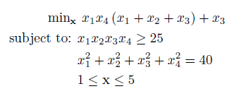
Consider the following problem from the NLP examples section:

To begin, we will enter it in mixed format:
fun = @(x) x(1)*x(4)*sum(x(1:3)) + x(3);
% Mixed Nonlinear Constraints
nlcon = @(x) [ prod(x); sum(x.^2) ];
nlrhs = [25;40];
nle = [1;0]; % [>=, =]
% Bounds (lb <= x <= ub)
lb = ones(4,1);
ub = 5*ones(4,1);
x0 = [1 5 5 1]';
% Build OPTI Object
Opt = opti('fun',fun,'nlmix',nlcon,nlrhs,nle,'bounds',lb,ub)
% Solve Problem
[x,fval] = solve(Opt,x0)
And again, lets repeat, this time in row format:
fun = @(x) x(1)*x(4)*sum(x(1:3)) + x(3);
% Row Nonlinear Constraints
nlcon = @(x) [ prod(x); sum(x.^2) ];
cl = [25;40];
cu = [Inf;40];
% Bounds (lb <= x <= ub)
lb = ones(4,1);
ub = 5*ones(4,1);
x0 = [1 5 5 1]';
% Build OPTI Object
Opt = opti('fun',fun,'nl',nlcon,cl,cu,'bounds',lb,ub)
% Solve Problem
[x,fval] = solve(Opt,x0)
As before, implemented correctly both methods will return the same result. Depending on the solver selected, it will present a warning if a conversion has taken place. Converting from mixed to row form is a simple conversion, as is from row to general form with only single bounds (each row only contains one inequality). Both of these conversions require no extra overhead while solving.
However, if you specify row constraints with dual bounds (two inequalities on one row) and OPTI is require to convert it to general form the overhead is substantially increased. Not only will the constraint function be modified, but also the Jacobian & Jacobian structure! Currently the Hessian is not modified, so be careful.
Summary
I am seeing more and more solvers using the row format for both linear and nonlinear constraints, so it may be worth considering adopting this format. Most LP solvers use the row format by default, while NLP solvers are split between each.