Supplying 1st Derivatives
Once you start solving real (differentiable) problems you will want to supply at least exact first derivatives. These can make a large difference (orders of magnitude) in the convergence, accuracy and computation time of the specified solver, when compared to numerical (finite-difference) derivatives.
This section will detail how to obtain exact first derivatives using OPTI and MATLAB, and how to supply them to the solver.
Mathematical Definition
Scalar Function
The first derivatives of a scalar, multivariable function f (such as that used in a NLP objective) is defined as:

Noting the result is a row vector, with dimensions 1 x n.
Vector Function
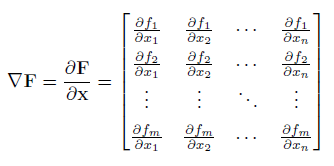
The first derivatives of a vector, multivariable function F (such as that used in a NLS objective, or vector of nonlinear constraints) is defined as:

Noting the result is a matrix, with dimensions m x n.
Naming Conventions
OPTI uses a fairly standard naming convention when referring to first derivatives.
Gradient
The gradient is always the first derivative of the objective function. It is identified by the keyword grad when supplying it as an argument to opti. Note the gradient is always dense, as all solvers supplied with OPTI expect it this way.
Jacobian
The Jacobian is always the first derivative(s) of the constraint function(s). It is identified by the keyword jac when supplying it as an argument to opti. The Jacobian may be dense or sparse, depending on the solver being used.
Strictly speaking a gradient should be a vector, while the Jacobian should be a matrix. However using these rules, argument names could be flipped based on the problem being solved! Therefore to keep things standard (and hopefully simple), the above naming strategy has been adopted where names are based on whether they refer to an objective, or constraint.
Example 1: Numerical Differentiation
As a baseline, let's consider the following scalar, multivariable nonlinear objective function from Hock & Schittkowski problem #71:

This can be created in MATLAB as follows:
fun = @(x) x(1)*x(4)*(x(1) + x(2) + x(3)) + x(3);
In order to numerically differentiate it, we will need to supply a point which we want to find the derivatives about. Then we can use the Intel djacobi method to solve for the first derivatives:
x0 = [1;2;3;4];
% Numerically Differentiate
df = mklJac(fun,x0)
This is the method that OPTI uses automatically if no derivatives are supplied, and the solver requires them. It has the advantage that it works with any function, even if it uses MATLAB Toolbox functions, MEX functions, or other black-boxes. However it is typically slower, and much less accurate than achievable via methods described below.
Example 2: Automatic Differentiation
One of the most widely used methods of supplying derivatives is via Automatic Differentiation (AD). It is used just like Numerical Differentiation (ND) above, but instead returns exact (to numerical precision) derivatives.
dfa = autoJac(fun,x0)
The OPTI autoJac function uses the ADIFF library to generate exact first derivatives. This is done using an object-orientated approach, overloading many common MATLAB operators and functions to calculate analytical first derivatives as it goes. ADIFF implements a forward AD algorithm, successively applying the chain rule to each operator / function it encounters.
While the AD library supplied with OPTI is fairly comprehensive in the functions it covers, it does not support 2D indexing, and thus is limited to relatively simple functions. It also does not support second derivatives (without running it twice), or automatically generate sparse representations, which several commercial tools do.
Example 3: Complex Step Differentiation
Another method for obtaining accurate derivatives is to use the complex-step method. This uses the built in complex number handling of MATLAB to accurately (to numerical precision) solve the first derivatives of a function.
dfc = cstepJac(fun,x0)
As with the automatic differentiation method, cstepJac only works on pure MATLAB functions. Also be careful with functions like abs, as well as relationship operators, as they are treated differently with complex numbers. In addition, watch out for using the complex conjugate operator (') rather than transpose (.'), this is the most common cause of errors with this function.
When used correctly complex step differentiation is faster than all other methods and provides derivatives accurate to numerical precision. It is however a little tricky to implement, given that the underlying function must be valid for complex numbers as well.
Example 4: Symbolic Differentiation
An alternative to computing derivatives at a point, during runtime, is symbolically calculate them once before solving, then supply them as complete functions to the solver. This requires a symbolic manipulator, and the MATLAB Symbolic Toolbox is used for this task.
grad = symJac(fun)
% Evaluate
dfs = grad(x0)
The above example shows how an anonymous function can be symbolically differentiated, then returned as a usable gradient function. It can then be evaluated at any point, and return an exact derivative.
The downside to this approach is that it can become very computationally expensive to evaluate the full derivative expression, especially second derivatives. On large, complex problems, ND or AD will be faster than evaluating the full, analytical expression.
Note the function symJac is a simple demonstration function for toy problems only. It is severly restricted in the problems it can process. However I am in the development of SymBuilder, currently included (but not well documented) in the OPTI distribution. This allows complex expressions to be symbolically processed and differentiated.
Example 5: Application to a NLP
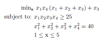
Now we have some tools for generating first derivatives, lets apply it to the full HS#71 NLP:

As done in previous examples, let's code it up in MATLAB:
fun = @(x) x(1)*x(4)*(x(1) + x(2) + x(3)) + x(3);
% Nonlinear Constraints
nlcon = @(x) [ x(1)*x(2)*x(3)*x(4);
x(1)^2 + x(2)^2 + x(3)^2 + x(4)^2 ];
cl = [25;40];
cu = [Inf;40];
% Bounds (lb <= x <= ub)
lb = ones(4,1);
ub = 5*ones(4,1);
% Initial Guess
x0 = [1 5 5 1]';
Now let's solve it using each of the strategies described so far to generate the first derivatives.
Numerical Differentiation
While done automatically by OPTI, it is explicity written out below.
grad = @(x) mklJac(fun,x);
% Jacobian
jac = @(x) mklJac(nlcon,x);
% Build OPTI Problem
Opt = opti('fun',fun,'grad',grad,'nl',nlcon,cl,cu,'jac',jac,...
'bounds',lb,ub,'x0',x0)
% Solve NLP
[x,fval,exitflag,info] = solve(Opt)
Automatic Differentiation
Forward AD in MATLAB:
grad = @(x) autoJac(fun,x);
% Jacobian
jac = @(x) autoJac(nlcon,x);
% Build OPTI Problem
Opt = opti('fun',fun,'grad',grad,'nl',nlcon,cl,cu,'jac',jac,...
'bounds',lb,ub,'x0',x0)
% Solve NLP
[x,fval,exitflag,info] = solve(Opt)
Complex Step Differentiation
Complex Step in MATLAB:
grad = @(x) cstepJac(fun,x);
% Jacobian
jac = @(x) cstepJac(nlcon,x);
% Build OPTI Problem
Opt = opti('fun',fun,'grad',grad,'nl',nlcon,cl,cu,'jac',jac,...
'bounds',lb,ub,'x0',x0)
% Solve NLP
[x,fval,exitflag,info] = solve(Opt)
Symbolic Differentiation
Note function handles are returned by symJac.
grad = symJac(fun);
% Jacobian
jac = symJac(nlcon);
% Build OPTI Problem
Opt = opti('fun',fun,'grad',grad,'nl',nlcon,cl,cu,'jac',jac,...
'bounds',lb,ub,'x0',x0)
% Solve NLP
[x,fval,exitflag,info] = solve(Opt)
Manual Differentiation
There is nothing stopping you entering the derivatives by hand!
grad = @(x) [x(1)*x(4) + x(4)*sum(x(1:3)), x(1)*x(4),...
x(1)*x(4) + 1, x(1)*sum(x(1:3))];
% Jacobian
jac = @(x) [prod(x')./x';
2.*x'];
% Build OPTI Problem
Opt = opti('fun',fun,'grad',grad,'nl',nlcon,cl,cu,'jac',jac,...
'bounds',lb,ub,'x0',x0)
% Solve NLP
[x,fval,exitflag,info] = solve(Opt)
Example 6: Exploiting Sparsity
For large-scale NLP solving it is typical the Jacobian will be quite sparse. For this reason large-scale NLP solvers (such as IPOPT and it's MI cousin BONMIN) expect the Jacobian to be sparse, as well as the user to supply the sparsity structure (indicating nonzero entries). Exploiting sparsity in this way can substantially improve the efficiency of the solver for large problems.
To supply a sparse Jacobian you can simply wrap your function handle in the sparse function:
jac = @(x) sparse([prod(x')./x';
2.*x']);
However this is not particularly efficient, as a sparse representation of the function will be generated at each function call. A more efficient method is to store it in the same way MATLAB does (sparse triplets), then convert it to the sparse datatype at the end. See the following MathWorks article on efficient handling of sparse matrices.
For the above problem you may note it is not rather sparse (in fact it is 100% dense), however it is just an example. Real examples of large scale nonlinear programming are too big to put here!
To generate the Jacobian structure callback, return a sparse matrix where a 1 indicates a nonzero entry, as follows:
jacstr = @() sparse(ones(2,4));
Note this function requires no input, as the structure is static. This means no matter what value of x, the structure should indicate all possible nonzero entries. It may be that nonzero entries change depending on x, however you must account for all possible entries in memory.
By default OPTI assumes the Jacobian Structure contains all ones, indicating a fully dense Jacobian. This is the most inefficient, but safest option.
Finally, to supply the entire problem to OPTI:
fun = @(x) x(1)*x(4)*(x(1) + x(2) + x(3)) + x(3);
% Gradient
grad = @(x) [x(1)*x(4) + x(4)*sum(x(1:3)), x(1)*x(4),...
x(1)*x(4) + 1, x(1)*sum(x(1:3))];
% Nonlinear Constraints
nlcon = @(x) [ x(1)*x(2)*x(3)*x(4);
x(1)^2 + x(2)^2 + x(3)^2 + x(4)^2 ];
cl = [25;40];
cu = [Inf;40];
% Jacobian
jac = @(x) sparse([prod(x')./x';
2.*x']);
% Jacobian Structure
jacstr = @() sparse(ones(2,4));
% Bounds (lb <= x <= ub)
lb = ones(4,1);
ub = 5*ones(4,1);
% Initial Guess
x0 = [1 5 5 1]';
% Options
opts = optiset('solver','ipopt','display','iter');
% Build OPTI Problem
Opt = opti('fun',fun,'grad',grad,'nl',nlcon,cl,cu,'jac',jac,'jacstr',jacstr,...
'bounds',lb,ub,'x0',x0,'options',opts)
% Solve NLP
[x,fval,exitflag,info] = solve(Opt)
You will note if you run the above example you will receive no warnings! You have now supplied the minimum amount of information required for OPTI to not make any assumptions to solve the problem using IPOPT.
Example 7: Checking Derivatives
It is all too easy to miss an index, be out by one, or any of the other common programming caveats. This is made even worse with large, sparse, partial derivative matrices! In order to check for errors, OPTI now comes with a derivative checker.
To activate it, enable the optiset option derivCheck:
opts = optiset('solver','ipopt','display','iter','derivCheck','on');
% Build OPTI Problem
Opt = opti('fun',fun,'grad',grad,'nl',nlcon,cl,cu,'jac',jac,'jacstr',jacstr,...
'bounds',lb,ub,'x0',x0,'options',opts)
% Solve NLP
[x,fval,exitflag,info] = solve(Opt)
If you examine the command window print out, you will see it says (for the above problem):
OPTI Derivative Checker detected no problems in 'Objective Gradient'
OPTI Derivative Checker detected no problems in 'Constraint Jacobian'
Indicating no errors were detected.
Summary
This section is a very brief introduction into generating first derivatives for optimization. However do not underestimate this topic, every gradient based optimizer in OPTI requires first derivatives. Just because OPTI will automatically approximate them using finite-difference does not mean you can ignore them!