OPTI Multi-Start Solver (multisolve)
The OPTI multi-start algorithm is a basic algorithm that repeatedly searches and optimizes the problem between the problem bounds, in order to avoid local minima. The algorithm is invoked using the following method:
where Opt is your OPTI optimization object. The algorithm is rather exhaustive and there is certainly room for improvement (anyone interested?). The algorithm so far is best explained using a plot:
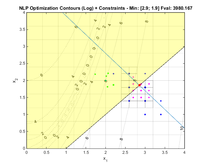
Referencing the plot above, the algorithm works as follows:
- The optimization problem is divided into equal sized regions (rectangles in 2D, boxes in 3D, and so forth) and the centre of each region is sampled. A score based on the objective and constraints is saved for each sample. (Phase 1)
- The local optimizer is run from the 10 best Phase 1 points (blue dots), within the bounds of the region of interest.
- The 5 best regions found are further sub-divided and sampled and a score recorded. (Phase 2)
- The local optimizer is run from the 10 best Phase 2 points (pink dots), once again within their respective region bounds.
- If x0 is supplied, a number of points are randomly scatted around it and a local optimizer run from each start point (green dots).
- The local optimizer runs a couple more times using heuristic based settings and the best solution returned (red dot).
Example 1: Non-convex QP
The following problem is a simple 2D QP - however it is a saddle point as the QP H matrix is indefinite. When solved normally (using solve) CLP will always return a solution at the bottom left of the plot below. However using multisolve, we can force it to find the global minimum (in this problem):
H = sparse([0 -1; -1 0]);
f = [0;0];
% Linear Constraints
lb = [-0.5;-0.5];
ub = [1;1];
% Options
opts = optiset('solver','clp','display','final');
% Build OPTI Object
Opt = opti('qp',H,f,'bounds',lb,ub,'options',opts)
% Solve Problem using MultiSolve
[x,fval,exitflag,info] = multisolve(Opt)
% Plot Problem + Search Area
multiplot(Opt)
Note the global minimum for this problem is at the top right, as found by multisolve:
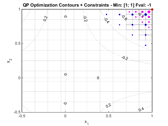
For more information on multiplot, see the plot examples page.
Example 2: Customizing the Search Area
Continuing from the above example, there may be times where you wish to increase or decrease the number of regions the algorithm searches in order to avoid skipping a solution. By default OPTI will always attempt to solve approximately 100 regions in Phase 1, but this is limited by the number of decision variables. The minimum 'division' per variable is 2, meaning the minimum number of points to search is 2^no_variables. You can see this algorithm is only applicable for small problems!
To increase the number search points, change the 3rd argument to multisolve (the second argument is x0, as per solve):
[x,fval,exitflag,info] = multisolve(Opt,[],30)
% Plot Problem + Search Area
multiplot(Opt)
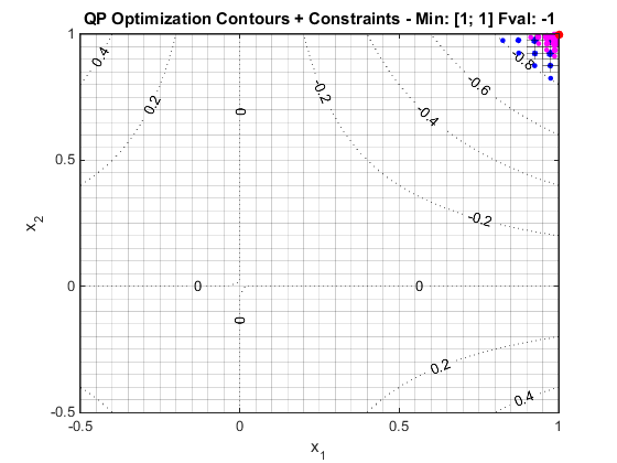
This time the plot below shows the Phase 1 regions (big boxes) have been divided into much finer search regions:
Example 3: Further Search Area Customization
As well as controlling the number of Phase 1 regions, you can also optionally specify the divisions for Phase 2. Simply supply a vector of the divisions to multisolve, as per the following example:
[x,fval,exitflag,info] = multisolve(Opt,[],[5 5])
% Plot Problem + Search Area
multiplot(Opt)
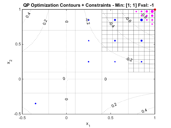
This time the plot below shows the Phase 2 regions (small boxes) have been divided into much finer search regions:
Example 4: Adjusting the Constraint Violation Penalty
Part of the search algorithm relies on adequately penalizing constraint violations. However determining an appropriate penalty weight has yet to be implemented, and is currently fixed at 1e4. This means if your objective function exceeds this value (approximately), it is unlikely the multi-start algorithm will pick the best points correctly.
To avoid this, the fourth argument to multisolve allows you to set this penalty value. An example of a value too low is shown below:
obj = @(x) (1-x(1))^2 + 100 *(x(2)-x(1)^2)^2;
% Linear Constraints
A = [-1 1]; b = -1;
Aeq = [1.1 1]; beq = 5;
lb = [0;0]; ub = [4;4];
% Initial Guess
x0 = [2;2];
% Options
opts = optiset('display','final');
% Build OPTI Object
Opt = opti('obj',obj,'ineq',A,b,'eq',Aeq,beq,'bounds',lb,ub,'options',opts)
% Solve Problem using MultiSolve and Lowered Penalty
[x,fval,exitflag,info] = multisolve(Opt,x0,[],100)
% Plot Problem + Search Area
multiplot(Opt,1)
The plot below shows the multi-start algorithm has decided to search within the infeasible region as although it is penalized, it is not as significant as being too far from the minimum. You will know when your penalty value is too low when the local optimizer is always infeasible.
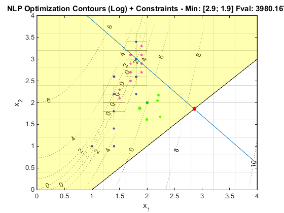
Note the converse is true as well, where over penalizing the constraints is also problematic.