Plotting OPTI Models
With the release of OPTI v2.00 comes more flexible plotting of optimization problems. You can now customize the generation of the plot, as well as being able to plot both 1D, and 3D-5D problems.
The basic command is:
where Opt is your OPTI optimization object. plot is for provided for quickly viewing your optimization problem, and not intended for paper quality plots.
Below are a few examples to get you familiar with the new functionality.
1D Plotting
A new feature of OPTI v2.00 is the ability to plot in 1D. 1D problems can be fairly 'academic', but let's look at plotting the Riemann Function (for details see the NLP Riemann Function Example):
fun = @RiemannND;
% Bounds
lb = 0.5; ub = 2;
% Starting Guess
x0 = 1;
% Options
opts = optiset('solver','nomad');
% Create OPTI Object
Opt = opti('fun',fun,'bounds',lb,ub,'x0',x0,'options',opts)
% Plot Problem
plot(Opt)
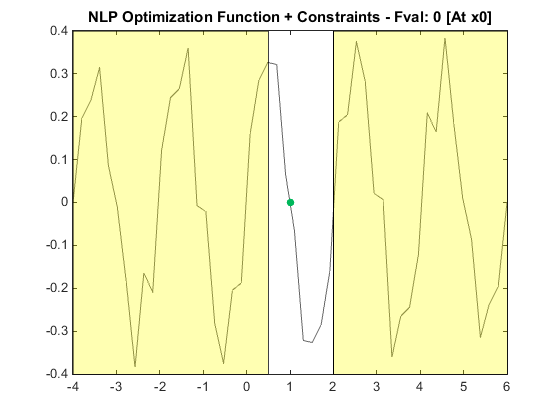
First thing you should notice is that we have plotted an unsolved problem! This is a new feature in v2.00, and allows plotting of problems which have x0, or are fully bounded. However the default plot settings leave a bit to be desired. Let's see what options we can play with:
plot Plot optimization problem (1D-5D only)
plot(optObj) plots the optimization field for the current
OPTI object.
plot(optObj,scale) plots with a user defined zoom level.
scale is defined as the range +- of the solution to be
drawn OR if supplied as a vector controls the bounds on the
plot [x1min x1max x2min x2max ... xNmin xNmax]
plot(obtObj,scale,dolog) plots the log of the objective
function (NL only)
plot(obtObj,scale,dolog,npts) controls the number of points
used for generating the objective and constraint contours
By examining the help we see we can better 'scale' the plot by providing both bounds on the plot axis limits. This effectively zooms the plot, but also increases the number of useful points used to generate the function:
plot(Opt,[lb ub])
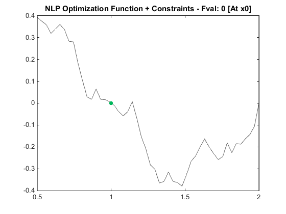
Now we are starting to get somewhere! However we are still lacking detail. This is where the npts argument comes in handy. It controls the number of points per variable that is used to generate function and constraint contours. By default it is around 50, let's try increasing it:
plot(Opt,[lb ub],[],1000)
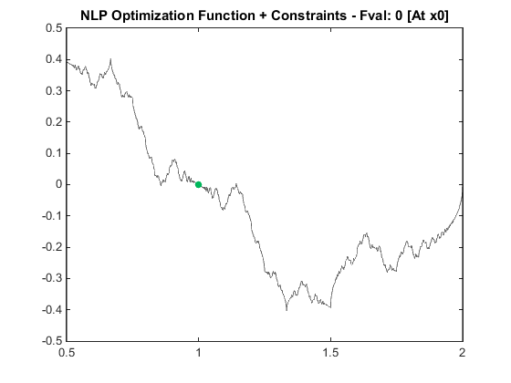
We now have a pretty good picture of the objective, and correct our initial guess to better setup the optimizer to solve this problem! Note 1000 is a really high number of points, typically 100-150 is sufficient (especially as it ends up as (ncon+1)*npts^ndec evals!):
[x,fval] = solve(Opt,1.4)
% Plot the Problem again, this time include solution
plot(Opt,[lb,ub],[],1000)
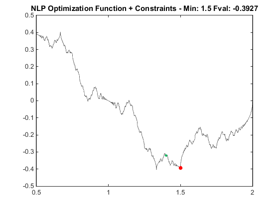
While still not the correct minimum, we have given NOMAD a fairly good chance of finding it given further customization of settings.
2D Plotting
Let's revisit some existing OPTI plotting functionality by plotting the Rosenbrock Banana Function:
fun = @(x) 100*(x(2) - x(1)^2)^2 + (1 - x(1))^2;
% Constraints
lb = [-5;-5]; ub = [5;5];
% Initial Starting Guess
x0 = [0;0];
% Setup Options
opts = optiset('solver','lbfgsb');
% Create OPTI Object
Opt = opti('fun',fun,'x0',x0,'bounds',lb,ub,'options',opts)
% Plot
plot(Opt)
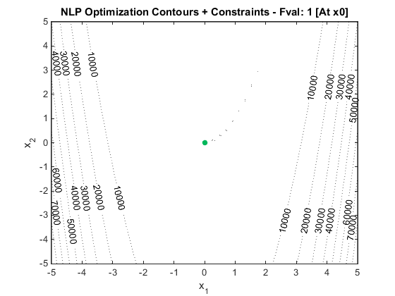
Looking at the above plot we either have a flat valley in the middle, or we are missing some detail! To get a better handle on the problem, lets zoom out a little so we can see the bounds as well:
plot(Opt,7)
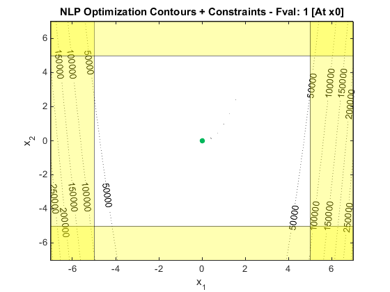
OK now we can see the region where we're expecting a solution, but we still can't see where that might be. Rather than pushing up the number of points used to draw the contours (as is done in the example above), lets take the log of the objective value:
plot(Opt,7,true)
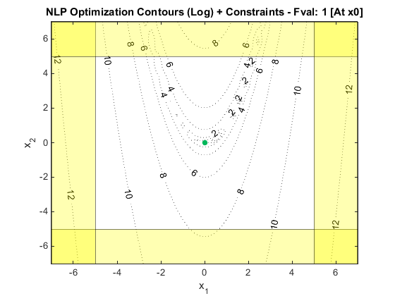
Now the familiar Rosenbrock function can be seen. I will leave you to experiment with various zoom and detail settings to see if you can find the optimum by inspection.
3D (and Higher) Plotting
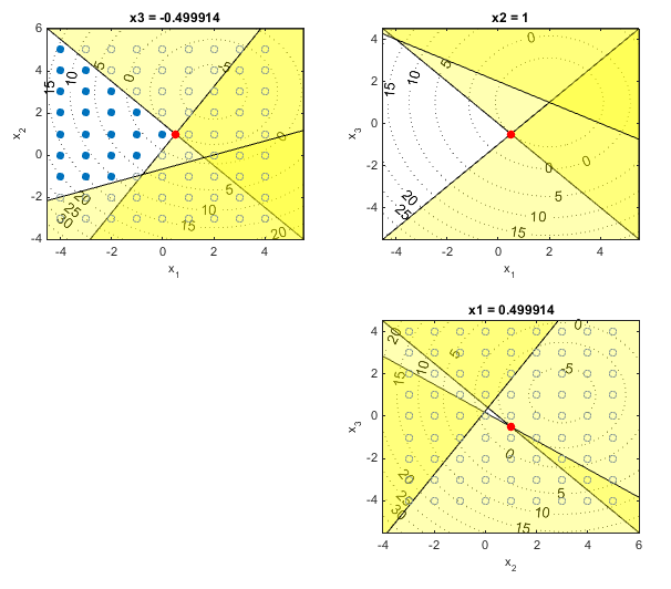
As well as 1D plotting, OPTI can now plot problems with up to 5 variables (5D). This is done by holding each variable constant, and plotting the other two in turn (or groups for higher orders). While not perfect, it does give you some insight into higher dimension problems and their structure!
Let us use the following 3D MIQP problem for example:
H = eye(3);
f = -[2 3 1]';
% Linear Constraints
A = [1 1 1;3 -2 -3; 1 -3 2];
b = [1;1;1];
% Integer Constraints
xtype = 'CIC';
%Build & Solve
Opt = opti('qp',H,f,'ineq',A,b,'xtype',xtype)
[x,fval,exitflag,info] = solve(Opt)
% Plot Problem
plot(Opt)
While the plots below are only valid for the solution point, they do show that the solution looks realistic:
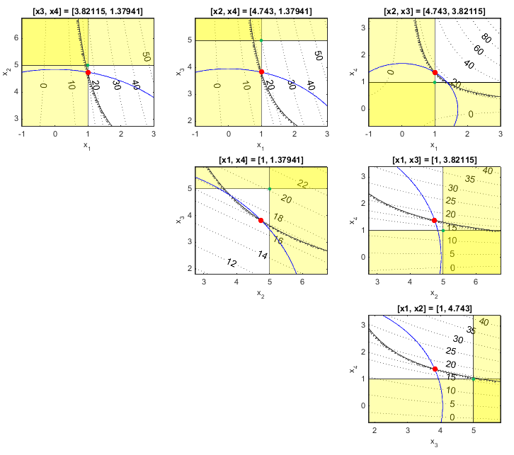
All the same options (scale,log,npts) are available for higher dimensional plotting, and OPTI manages all the hard work for you. For more examples see test_3dplots.m supplied with OPTI. Below is an example of a 4D plot of Hock & Schittkowski #71:
Plotting MultiSolve Solutions
Another new feature in v2.00 is the multisolve function, which is a simple implementation of a multi-start solver. In addition to being able to plot the solution of a multisolve run (as per above examples), a new function multiplot is also available, which shows where OPTI has searched and evaluated your problem.
multiplot has the same functionality as plot, except it does not provide the scale argument (it always plots between problem bounds). Below is an example solving the Rosenbrock problem with a couple additional linear constraints:
obj = @(x) (1-x(1))^2 + 100 *(x(2)-x(1)^2)^2;
% Linear Constraints
A = [-1 1]; b = -1;
Aeq = [1.1 1]; beq = 5;
lb = [0;0]; ub = [4;4];
% Initial Guess
x0 = [2;2];
%Build & Solve using multiplot
Opt = opti('obj',obj,'bounds',lb,ub,'ineq',A,b,'eq',Aeq,beq)
[x,fval,ef,info] = multisolve(Opt,x0)
% Plot Problem using multiplot and take log(obj)
multiplot(Opt,1)
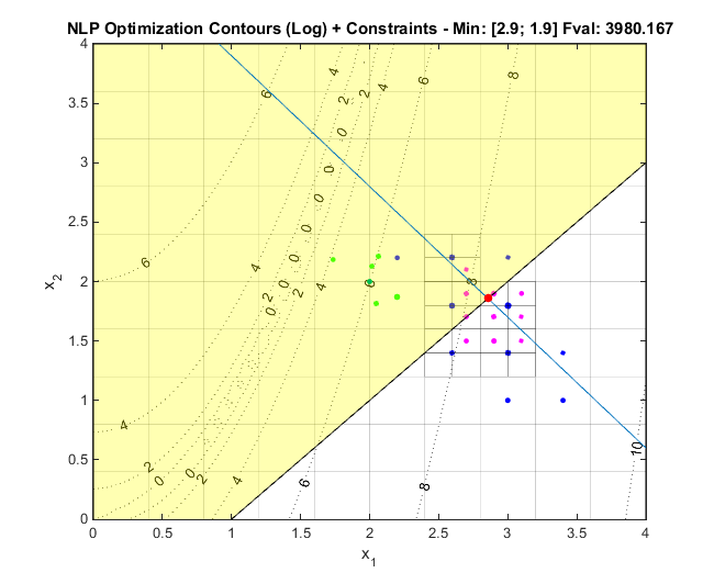
The plot below shows the gridded area of where OPTI has searched. Blue points represent the best points found in Phase 1, pink points best in Phase 2. Green points are the initial guess points.
Summary
While plotting objective problems may actually take longer than solving them, it is still useful to gain an understanding of what your problem actually looks like. Just remember to use the extra arguments to plot to get a better view of the problem!