OPTI Toolbox

Problem Definition

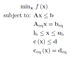
An GNLP has the following form:

Where f is a scalar function containing the nonlinear objective function, which is subject to the following constraints:

Linear Inequalities*

A is a m x n sparse matrix, b is a m x 1 vector.

Linear Equalities*

A_eq is a k x n sparse matrix, b_eq is a k x 1 vector.

Decision Variable Bounds

l_b and u_b are n x 1 vectors, where -inf or inf indicate an unbounded lower or upper bound, respectively.

Nonlinear Inequalities*

c is a u x 1 vector of functions containing nonlinear inequality constraints, d is a u x 1 vector

Nonlinear Equalities*

c_eq is a v x 1 vector of functions containing nonlinear equality constraints, d_eq is a v x 1 vector

The goal is to minimize the objective function by selecting a value of x that also satisfies all constraints.

*Your problem description will either use Linear / Nonlinear Inequalties and Linear / Nonlinear Equalities OR Linear / Nonlinear Row Constraints. See the constraint information page.

Note an GNLP is created in the exact same way as an NLP. It is recommened you complete reading the NLP section before reading the remainder of the section.

GNLP vs NLP

You may have noticed the defintion of a GNLP is exactly the same as a NLP. Well in fact it is (in my terminology), what varies is the how the solver works, and the type of solution returned.

A global solver will attempt to find the global optimum to a problem, which may be significantly different from a local solution. There are multiple strategies to do this, however they fall into two general categories: derivative based and derivative free.

Derivative Based Global Optimizers

Global optimizers which use derivatives must use extra information, other than just the derivatives, in order to find a solution, otherwise they would fall into the same local minima. Typically a white-box model is required, where the model, including all the equations, is passed directly to the solver. This allows the optimizer to exploit the structure of the system in order to find a global solution, typically using a cutting plane based approach together with branch and bound.

As of OPTI v1.73 SCIP has been updated to allow it to solve NLPs and MINLPs to global optimality. The interface parses your MATLAB functions into an algebraic description, which is then used by the solver, see the White Box Optimization page for more details. In addition, from OPTI v2.05 the global optimization solver BARON is also interfaced. There is also an open-source project, Couenne, which implements this functionality, but I have not had the time to write an interface for it.

An alternative to the white-box approach is multi-start. This runs a local optimizer over many initial start points, and returns the best solution from all runs. The multisolve algorithm supplied with OPTI provides a very basic implementation of a multi-start solver.

Derivative Free Global Optimizers

Derivative free optimizers use strategies like direct search, particle swarm, ant colony, and genetic algorithm to solve the problem. These solvers require no derivative information, and instead only require objective and constraint evaluations. The downside is they will typically use many more function evaluations in order to find a solution.

Derivative free optimizers are also suited to general NLP problems, where the objective or constraints may be non-differentiable, or subject to stochastic noise. An example is fitting parameters to an ODE, when using an adaptive step-size integrator.

OPTI includes a number of derivative free, global optimizers, including NOMAD (my favourite), PSwarm (parallelizable) and global solvers within NLopt.

Example 1: Small GNLP

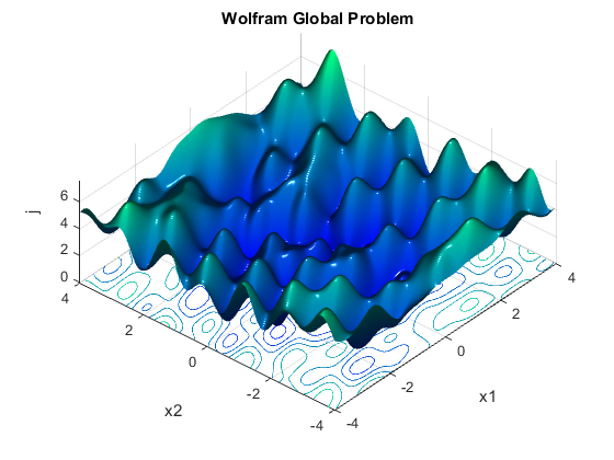
Lets revisit the non-convex problem from the NLP section:

Previously we attempted to solve this problem using IPOPT, a local optimizer. Let's compare IPOPT's solution with those obtained from a selection of global optimization routines:

Note in this example we have used the intermediate function optiprob to create a common problem structure. The syntax for this function is the same as for opti, and can be more useful for larger problem descriptions.

Now let's solve each problem, and see what results we got:

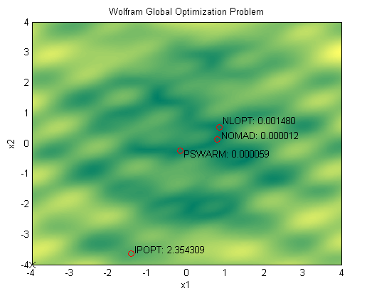
The above plot shows each optimizer has in fact returned a different solution. Remember this problem has multiple global minima at fval = 0, thus solutions obtained by NOMAD and PSwarm appear valid (within the default tolerances). NLopt has found a reasonable solution, while IPOPT has fallen into a local minima, as expected.

You may obtain different results from PSwarm as it uses a randomizing pattern as part of it's algorithm. The other solvers are all deterministic.

Example 2: Non-convex Polynomial

The following example is a 6th order polynomial bounded between -1.5 and 1.5:

For this problem we will use a new feature of OPTI (starting from v1.73) which allows general MATLAB functions to be parsed into an algebraic description and then solved using SCIP. This allows SCIP to solve general NLPs and MINLPs to global optimality, provided an algebraic description of the system can be generated. The following code shows how SCIP can be substituted as the NLP solver and called just like any other NLP or GNLP solver:

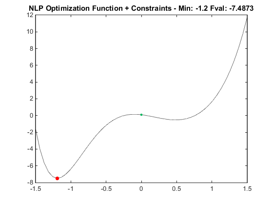
Using SCIP the above code will find the global minimum at x = -1.19, while local solvers such as IPOPT will typically get stuck in the local minimum at x = 0.486. Obviously moving x0 will closer to the optimum will help local solvers, but this is not so easy to see in higher dimensions!

The new SCIP interface will parse any normal MATLAB function (or anonymous function) as long as the functions are limited exp, log, log10, abs, and sqrt. In addition, your function must be deterministic (no random or stochastic elements), and must not use any relational operators or trigonometric functions. Indexing and vectorizing up to 2D is supported. See the White Box Optimization page for more examples.