Linear Program (LP)
Problem Definition
An LP has the following form:
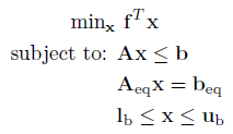
Where f is a n x 1 vector containing the linear objective function, which is subject to the following constraints:
Linear Inequalities*
A is a m x n sparse matrix, b is a m x 1 vector.
Linear Equalities*
Aeq is a k x n sparse matrix, beq is a k x 1 vector.
Decision Variable Bounds
lb and ub are n x 1 vectors, where -inf or inf indicate an unbounded lower or upper bound, respectively.
The goal is to minimize the objective function by selecting a value of x that also satisfies all constraints.
*Your problem description will either use Linear Inequalties and Linear Equalities OR Linear Row Constraints. See the constraint information page.
Example 1: Small Dense LP
Consider the following LP from the basics section:
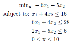
Note two important characteristics of this problem which make it an LP:
- The objective function is linear (the only operation is a constant times each decision variable, and the result summed).
- The constraints are also linear, as above.
Because of this linear property, we can rewrite this problem in matrix-vector form:
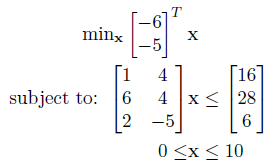
And supply the entire problem to the solver as a collection of matrices and vectors. This not only avoids costly callbacks to MATLAB, but the solver also knows the full structure of the model which it can use when solving.
Using the native matrix & vector notation of MATLAB this can be entered as so:
f = -[6 5]'; %Objective Function Vector (min f'x)
% Constraints
A = [1,4; 6,4; 2,-5]; %Linear Inequality Constraints (Ax <= b)
b = [16;28;6];
lb = [0;0]; %Bounds on x (lb <= x <= ub)
ub = [10;10];
And the problem solved by passing the problem variables to OPTI, and calling solve on the resulting object:
Opt = opti('f',f,'ineq',A,b,'bounds',lb,ub)
% Solve the LP problem
[x,fval,exitflag,info] = solve(Opt)
Because the problem contains only two variables, we can use OPTI's built in plot command to view the solution:
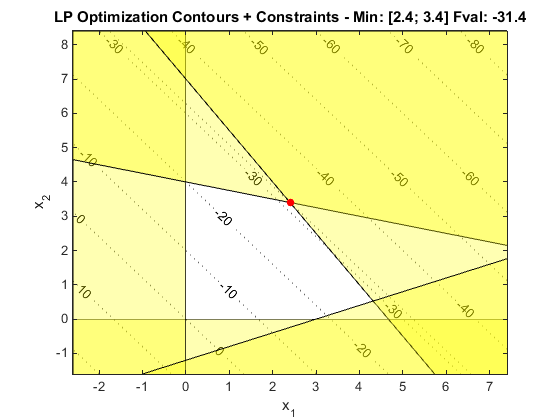
You can see from the above figure that the linear gradient of the objective (dashed in grey) as well as the inequality constraints. Shaded areas represent infeasible regions. As with all LPs the solution will lie on a constraint, or intersection of one or more constraints. For LPs the objective gradient will always be equally spaced straight dashed lines, and constraints straight lines.
Example 2: Large Sparse LP
The above example represents the 'toy' problems that are common when learning linear programming. In reality the problems will typically contain hundreds of decision variables and thousands of constraints. In order to efficiently solve these problems the sparsity structure of the inequality and equality constraints must be exploited.
To illustrate, load a large LP supplied as a .MPS problem with OPTI and lets examine the A matrix:
prob = coinRead('maros-r7.mps')
% Examine A matrix
spy(prob.A)
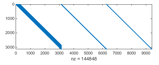
The figure generated shows just how sparse the matrix is, with less than 0.5% of the entries containing a value other than zero. Exploiting sparsity means ignoring all the values which are zero, both when storing and solving the problem. This saves a lot of memory, and computation time!
In fact the preferred format for LPs with OPTI is to use the MATLAB sparse data type. This is due to all LP solvers supplied with OPTI accepting sparse constraints only! If you supply a dense matrix, it will be automatically converted to a sparse representation. Note the objective vector f and constraint upper and lower bounds, rl and ru must remain dense vectors.
The next important point with the loaded model is the representation of constraints. So far I have shown constraints where the inequality and equality constraints are stored and supplied separately. While this is the MATLAB default, a more efficient method is to store in what I call 'row format', as follows:

This format places bounds on each row of the constraint matrix A. See the constraint information page for more information on this format.
Finally to solve this problem, consider the format the problem has been loaded in:
This structure is a OPTI generated structure that contains all information required to define an optimization problem. It is a standard MATLAB structure so you are free to process it how you like, but it can also be supplied to OPTI as is:
Opt = opti(prob)
% Solve the resulting model
[x,fval] = solve(Opt);
Example 3: LP in Row Format
Consider the following toy LP problem:
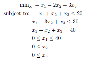
For this problem we are going to enter it to OPTI in row format. You are free to choose the format, however you cannot mix the two in one problem. You will be presented with a warning if the selected solver requires a different format (warning level dependent).
f = -[1 2 3]';
% Row Constraints (rl <= A*x <= ru)
A = sparse([-1 1 1; %sparse even though all nz
1 -3 1;
1 1 1]);
rl = [-Inf;-Inf;40]; %top two rows are only Ax <= b
ru = [20;30;40];
% Bounds (lb <= x <= ub)
lb = [0;0;0];
ub = [40;Inf;Inf]; %x2 and x3 are unbounded above
% Setup Options
opts = optiset('solver','clp'); %CLP is a row constraint solver
% Build OPTI Object
Opt = opti('f',f,'lin',A,rl,ru,'bounds',lb,ub,'options',opts)
% Solve Problem
[x,fval] = solve(Opt)
Example 4: LP with 'Mixed' Constraints
Keeping with the same LP with from Example 3, we are going to enter it in a seldom used, but sometimes useful format I've called 'mixed'. This is identical to how nonlinear constraints can be specified, described here. Basically 3 argument are supplied where A and b are as per the problem definition except e allows a change of constraint type. -1 corresponds to <=, 0 to == (equality) and 1 to >=.
f = -[1 2 3]';
% Linear Constraints
A = sparse([-1 1 1; %sparse even though all nz
-1 3 -1; %note this row inverted just for example purposes
1 1 1]);
b = [20;-30;40];
e = [-1;1;0]; %-1 <=, 0 ==, 1 >=
% Bounds (lb <= x <= ub)
lb = [0;0;0];
ub = [40;Inf;Inf]; %x2 and x3 are unbounded above
% Setup Options
opts = optiset('solver','clp'); %CLP is a row constraint solver
% Build OPTI Object
Opt = opti('f',f,'mix',A,b,e,'bounds',lb,ub,'options',opts)
% Solve Problem
[x,fval] = solve(Opt)
Example 5: Adding a Constant Objective Bias
Consider the following alternative objective definition for an LP:

Sometimes I get asked how to enter an LP (or MILP or QP) with a constant objective term. In fact it actually makes no difference to the solution vector x when solving these problems! The only difference is the returned fval will not be offset by this bias. However from OPTI v2.00 you can now enter this bias as part of the problem description:
f = -[6 5]';
objbias = 5;
% Linear Constraints (A*x <= b)
A = [1,4; 6,4; 2, -5];
b = [16;28;6];
% Bounds (lb <= x <= ub)
lb = [0;0]; ub = [10;10];
% Build OPTI Object
Opt = opti('f',f,'objbias',objbias,'ineq',A,b,'bounds',lb,ub)
% Solve Problem
[x,fval] = solve(Opt)
You will note that no matter what the value of objbias is, the same solution is returned in x. Most solvers accept the constant bias as part of the problem description, thus iteration print out will reflect the bias as well. Solvers that do not accept the bias will have it manually added after it has completed solving.
The constant objective bias term is only available for (MI) LP, QP and SDP problems. The bias has also been added to the File IO routines so you can read and write mathematical files with this constant.