OPTI Toolbox

Problem Definition

An MILP has the following form:

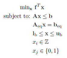
Where f is a n x 1 vector containing the linear objective function, which is subject to the following constraints:

Linear Inequalities*

A is a m x n sparse matrix, b is a m x 1 vector.

Linear Equalities*

A_eq is a k x n sparse matrix, b_eq is a k x 1 vector.

Decision Variable Bounds

l_b and u_b are n x 1 vectors, where -inf or inf indicate an unbounded lower or upper bound, respectively.

Integer Constraints

x_i are decision variables which must be an integer number (..-2, -1, 0, 1, 2..).

Binary Constraints

x_j are decision variables which must be a binary number (0,1), where i ≠ j.

The goal is to minimize the objective function by selecting a value of x that also satisfies all constraints.

*Your problem description will either use Linear Inequalties and Linear Equalities OR Linear Row Constraints. See the constraint information page.

Note an MILP is created in the same way as an LP, except some variables are defined to take discrete (integer) values only. It is recommened you complete reading the LP section before reading the remainder of the section.

Example 1: Small Dense MILP

Consider the following LP from the basics section, modified as an MILP:

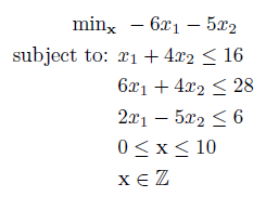
Using the native matrix & vector notation of MATLAB this can be entered as so:

And the problem solved by passing the problem variables to OPTI, and calling solve on the resulting object:

Because the problem contains only two variables, we can use OPTI's built in plot command to view the solution:

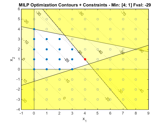
You can see from the above figure that the linear gradient of the objective (dashed in grey) as well as the inequality constraints. Shaded areas represent infeasible regions. Unlike an LP, the optimum may not lie on a constraint, where the blue dots indicate feasible integer solutions. Note the Mixed Integer (MI) optimum is different to the relaxed (LP) optimum from the previous example, which is generally the case.

Example 2: Alternative Integer Setup

There are two ways integer variables can be declared to the OPTI object constructor.

Character String

Supply a string of characters representing C (continuous), B (binary) and I (integer):

Index Vector

Supply a double vector of the indicies of the integer variables:

Note that with this method, only integer variables can be defined (not binary). However you can manually add bounds to enforce a binary variable, if required.

Example 3: Sparse MILP

As with LPs the Example 1 is a toy problem, and real MILP problems will be orders of magnitude bigger. In order to efficiently solve these problems the sparsity structure of the inequality and equality constraints must be exploited.

To illustrate, load a MILP supplied as a .MPS problem with OPTI and lets examine the A matrix:

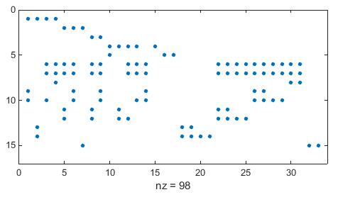
While not as sparse as the previous LP example, this problem still contains less than 19% nonzero entries.

To solve this problem, pass the loaded problem structure to the OPTI constructor:

Example 4: MILP with Special Ordered Set (SOS)

Consider the following MILP problem:

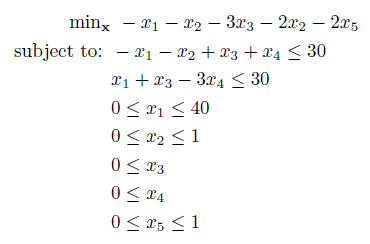
Initially this problem looks like an LP, however we are going to add one more constraint. We are going to specify that only one variable from x₁ to x₅ can take on a nonzero value. This type of constraint could be used when choosing one option from a selection.

To model this constraint, we could either introduce binary variables and add the required constraints, or we can specify it as a SOS of type 1. For more information on SOS, consult the SOS section.

Note from OPTI v1.81 the names of SOS structure fields has changed. However you can still enter individual arguments, as is done below:

You will have noticed the introduction of a SOS told OPTI this was a MILP. However we did not need to add any binary variables (or variable types for that matter), and our problem description remains succinct. SOS are also typically handled more efficiently by solvers than if you were to manually include binary variables and constraints, and you can add as many sets as you want!

To add multiple SOS constraints, follow the below construction:

Note using the above construct we are utilizing the new SOS API, whereby a single structure is supplied with the fields 'type', 'index', and 'weight'. This API can be used for both single and multiple SOSs, noting cell arrays are used for indices and weights when specifying multiple SOSs. In the above example, we are effectively telling the optimizer to choose one variable between index 1 and 2, and two variables between index 3 and 5.

Example 5: Specifying Long Integer Variable Strings

A common question we get is how to specify xtype when you have lots of integer variables. Assuming your variables are ordered (i.e. continuous, integer and binary variables are in consecutive groups), the following example shows a shorthand trick to enter them.

Summary

While the algorithms for solving MILPs have advanced tremendously in the past couple of decades, these are still complex problems and will take much more time than a LP to solve. They also scale poorly with size, so using a commercial solver such as CPLEX which exploits multicore processors can be a significant advantage.

Also note the solution obtained from a MILP solver may not be the global minimum as integer constraints make the problem non-convex.