Nonlinear Program (NLP)
Problem Definition
An NLP has the following form:
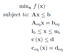
Where f is a scalar function containing the nonlinear objective function, which is subject to the following constraints:
Linear Inequalities*
A is a m x n sparse matrix, b is a m x 1 vector.
Linear Equalities*
Aeq is a k x n sparse matrix, beq is a k x 1 vector.
Decision Variable Bounds
lb and ub are n x 1 vectors, where -inf or inf indicate an unbounded lower or upper bound, respectively.
Nonlinear Inequalities*
c is a u x 1 vector of functions containing nonlinear inequality constraints, d is a u x 1 vector
Nonlinear Equalities*
ceq is a v x 1 vector of functions containing nonlinear equality constraints, deq is a v x 1 vector
The goal is to minimize the objective function by selecting a value of x that also satisfies all constraints.
*Your problem description will either use Linear / Nonlinear Inequalties and Linear / Nonlinear Equalities OR Linear / Nonlinear Row Constraints. See the constraint information page.
Example 1: Small NLP
Consider the following NLP:

Note two important characteristics of this problem which make it an NLP:
- The objective function contains a nonlinear operator (
log) - The constraint contains a quartic
As both the objective and constraint are nonlinear, they must be written as general functions. These can either be anonymous functions (as below), or MATLAB functions in their own M-file.
The big disadvantage with an NLP is that now these functions are 'black-boxes', the optimizer does not know the function nor it's structure, hence these problems are significantly more difficult than LPs or QPs.
fun = @(x) log(1 + x(1)^2) - x(2); %Objective Function Vector (min f(x))
% Nonlinear Constraints
nlcon = @(x) (1 + x(1)^2)^2 + x(2)^2; %Nonlinear Equality Constraint
nlrhs = 4;
nle = 0; %Constraint type: -1 <=, 0 ==, 1 >=
The problem is solved by passing the problem variables to OPTI, and calling solve on the resulting object:
Opt = opti('fun',fun,'nlmix',nlcon,nlrhs,nle,'ndec',2)
% Solve the NLP problem
x0 = [2;2] %Initial Guess
[x,fval,exitflag,info] = solve(Opt,x0)
Because the problem contains only two variables, we can use OPTI's built in plot command to view the solution:
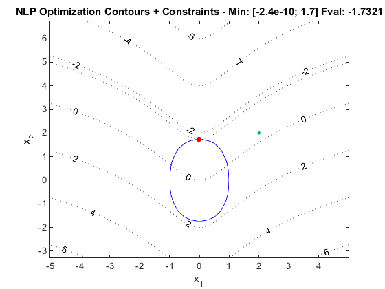
As shown the optimizer has found a solution on the equality constraint (blue). We have supplied the minimum amount of information to solve this problem, thus OPTI has made a number of assumptions and approximations, and you may be presented with a number of warnings (set optiset option 'warnings' to 'all' to see assumptions).
Note the argument 'ndec' supplied to opti is only required when OPTI cannot determine the number of decision variables passed to the constructor. In this problem all arguments are function handles, or related to the constraints, thus ndec cannot be determined, and is required to perform test evaluations. If you supply bounds, a starting guess, gradient, Hessian or integer variable declaration this argument is not required.
Example 2: Multiple Nonlinear Constraints
When solving NLPs it is common that you will have more than one nonlinear constraint. A common test problem is the Hock & Schittkowski #71, described below:
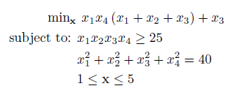
To enter this problem into OPTI, all constraints must supplied as a single vector function, as follows:
fun = @(x) x(1)*x(4)*(x(1) + x(2) + x(3)) + x(3);
% Nonlinear Constraints (cl <= nlcon(x) <= cu)
nlcon = @(x) [ x(1)*x(2)*x(3)*x(4);
x(1)^2 + x(2)^2 + x(3)^2 + x(4)^2 ];
cl = [25;40];
cu = [Inf;40];
% Bounds (lb <= x <= ub)
lb = ones(4,1);
ub = 5*ones(4,1);
% Initial Guess
x0 = [1 5 5 1]';
% Options
opts = optiset('solver','ipopt','display','iter');
% Build OPTI Problem
Opt = opti('fun',fun,'nl',nlcon,cl,cu,'bounds',lb,ub,'x0',x0,'options',opts)
% Solve NLP
[x,fval,exitflag,info] = solve(Opt)
Note in this example I have entered the constraints in row format, but this is not required for multiple constraints. Either mixed (as per the problem definition above) or row format is typically fine.
If you have a large number of nonlinear constraints to define, but the constraints share a common structure, have a look here for ideas on how to automate building them.
Example 3: Linear Constraints
Apart from the MATLAB Optimization Toolbox solvers, the remaining OPTI NLP solvers (with the exception of SCIP) do not distinguish between linear constraints and nonlinear constraints when building or solving the problem. If you supply linear constraints, OPTI will automatically convert them to nonlinear form, and either supply them to the solver, or append them to the existing nonlinear constraints.
In saying that, IPOPT does have an option to indicate all inequality or equality constraints are linear. Consider the following NLP with linear constraints:

This can be solved using IPOPT as follows:
fun = @(x) (x(1) - x(2))^2 + (x(2) + x(3) - 2)^2 + (x(4) - 1)^2 + (x(5) - 1)^2;
% Linear Equality Constraints
Aeq = [1 3 0 0 0;
0 0 1 1 -2;
0 1 0 0 -1];
beq = [4;0;0];
% Starting Guess
x0 = [ 2.5 0.5 2 -1 0.5 ];
% Options
opts = optiset('solver','ipopt');
% Create OPTI Object
Opt = opti('fun',fun,'eq',Aeq,beq,'options',opts)
% Solve using IPOPT
[x,fval,exitflag,info] = solve(Opt,x0)
If you examine the returned info structure, it contains a field called FuncEvals. The property Jacobian is set to 1, indicating IPOPT only did one Jacobian evaluation. OPTI has automatically identified all constraints are linear, and set the corresponding option in IPOPT, allowing it to avoid multiple Jacobian evaluations.
However, if one inequality or equality constraint is nonlinear, the entire Jacobian must be evaluated at each call.
Example 4: Unconstrained Nonlinear Optimization
An alternative to an NLP is an Unconstrained Nonlinear Optimization (UNO) problem. These problems contain no linear, nonlinear or bound constraints, and thus only a objective function is required.
An example is the classic Rosenbrock function:

This can be solved using OPTI as follows:
fun = @(x) 100*(x(2) - x(1)^2)^2 + (1 - x(1))^2;
% Starting Guess
x0 = [0;0];
% Create OPTI Object
Opt = opti('fun',fun,'x0',x0)
% Solve
[x,fval,exitflag,info] = solve(Opt)
Note in this example we have supplied x0 to the opti constructor, so it is stored as part of the problem. This prevents the need to supply ndec to tell OPTI how many decision variables the problem has.
While UNO problems are fairly common, I highly recommend at least upper and lower bounds are placed on all variables. This aids the solver in scaling the variables, as well as providing a known search space.
Example 5: Supplying Derivatives
So far all examples have automatically utilized Intel's djacobi routine, (implemented in OPTI as mklJac) for approximating both the objective and constraint derivatives via finite differences. While this works OK for small, well behaved problems, real problems you will want to implement your own, exact, derivatives.
Note there are two detailed sections on this topic, 1st Derivatives and 2nd Derivatives, however a small problem will be presented here.
Consider the same problem from Example 1, however this time we will supply exact first derivatives:
fun = @(x) log(1 + x(1)^2) - x(2);
% Objective Gradient (row vector)
grad = @(x) [2*x(1)/(x(1)^2+1) -1];
% Nonlinear Constraints
nlcon = @(x) (1 + x(1)^2)^2 + x(2)^2;
nlrhs = 4;
nle = 0;
% Constraint Jacobian (matrix, one row per constraint)
jac = @(x) [4*x(1)*(x(1)^2+1), 2*x(2)];
Adding first derivative information to OPTI is easy, just tag on the extra arguments:
Opt = opti('fun',fun,'grad',grad,'nlmix',nlcon,nlrhs,nle,'jac',jac,'ndec',2)
% Solve the NLP problem
x0 = [2;2] %Initial Guess
[x,fval,exitflag,info] = solve(Opt,x0)
Example 6: Differentiability, Convexity, and Local Solutions
Apart from a few specialized OPTI solvers (NOMAD, PSwarm, some NLOPT solvers - i.e. GNLP solvers), the remaining NLP solvers require your objective and constraints to be:
- Smooth and twice differentiable (no noise, stochastic or pathological problems)
- Convex (if not, only local solutions may be found)
Non-Differentiable Function
Consider the single dimension Riemann function below (from Wolfram):
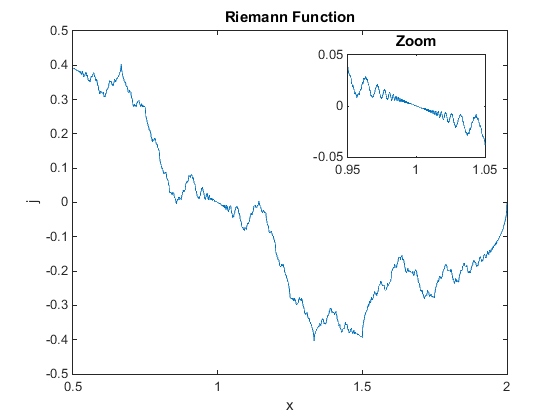
This function has a particularly nasty property that makes it non-differentiable, meaning our gradient based optimizers (IPOPT, L-BFGS-B, etc) will have a hard time! It is also horribly nonconvex! The global optimum (within the bounds of the plot) is at x = 1.333.
Create a m-file function with the following code:
% Riemann's non-differentiable function, R(x) for rational x = p/q
[p,q] = rat(x);
R = 0;
for k = 1:q-1
R = R + sin(k^2*p*pi/q)/(sin(k*pi/2/q))^2;
end
R = R*pi/4/q/q;
end
Now let's attempt to solve it using IPOPT:
fun = @RiemannND;
% Bounds
lb = 0.5;
ub = 2;
% Starting Guess
x0 = 1;
% Options
opts = optiset('solver','ipopt');
% Create OPTI Object
Opt = opti('fun',fun,'bounds',lb,ub,'options',opts)
% Attempt to Solve
[x,fval,exitflag,info] = solve(Opt,x0)
On my PC IPOPT returned in 6 seconds with x = 0.5. Changing the starting guess to x0 = 1.5, and it hadn't returned after 180 seconds. Considering we are only solving a 1D problem, these solve times are significant. Note as the problem is not differentiable, OPTI is using a finite difference approach to obtain the objective gradient, which will be returning nonsense.
Therefore problems like these cannot be solved using gradient based optimizers like IPOPT, LBFGSB, and others. Consider using a Global solver such as NOMAD.
Non-Convex Function
Another difficult problem is the non-convex problem. Note in this case the problem is differentiable, but due to the model structure and functions, multiple minima exist.
Consider the following two dimensional function below (from Wolfram):
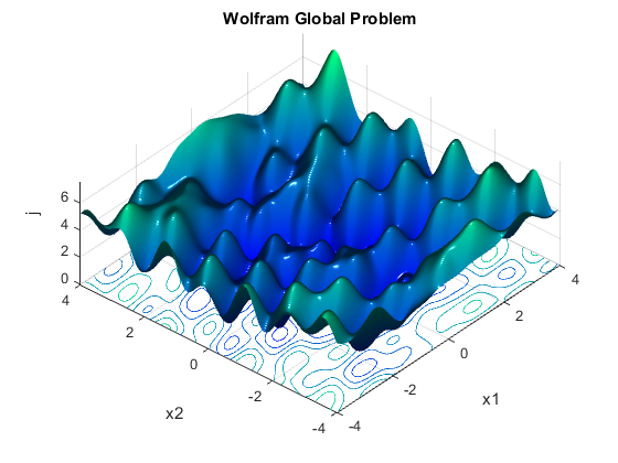
In reality, this problem has multiple global optima which is unusual, however there are also multiple local minima. The global optimum is fval = 0. This problem has been converted from a Nonlinear Least Squares (NLS) problem to a NLP by taking the norm of the vector of fitting functions (yes it should be the norm2), as follows:
ffun = @(x) [x(1) - sin(2*x(1) + 3*x(2)) - cos(3*x(1) - 5*x(2));
x(2) - sin(x(1) - 2*x(2)) + cos(x(1) + 3*x(2))];
% Objective
fun = @(x) norm(ffun(x));
Now let's attempt to solve it using IPOPT:
lb = [-4;-4];
ub = [4;4];
% Starting Guess
x0 = [0;-3];
% Options
opts = optiset('solver','ipopt');
% Create OPTI Object
Opt = opti('fun',fun,'bounds',lb,ub,'options',opts)
% Attempt to Solve
[x,fval,exitflag,info] = solve(Opt,x0)
This time IPOPT solved much faster (as expected), but the solution returned is a local minima. IPOPT has also incorrectly reported it as the optimum solution. This is due to IPOPT being a local solver, meaning for non-convex problems it will return the first minima it finds. For convex problems (where the local minimum = the global minimum), the result returned will always be the actual optimum (if a feasible solution is found).
You can read more about convex problems at Wikipedia, Frontline and an excellent PDF from the makers of CVX - a convex optimization package.