OPTI Toolbox

Note from OPTI v2.10 a new API exists via optifit which simplifies the construction and solving of curve and surface fitting problems. However for more complex problems, or for more control of the solving process, the below methods are still recommended.

Problem Definition

An NLS has the following form:

Where F is a vector function containing the nonlinear fitting function, and ydata is the fitting data, which is subject to the following constraints:

Linear Inequalities

A is a m x n dense matrix, b is a m x 1 vector.

Linear Equalities

A_eq is a k x n dense matrix, b_eq is a k x 1 vector.

Decision Variable Bounds

l_b and u_b are n x 1 vectors, where -inf or inf indicate an unbounded lower or upper bound, respectively.

The goal is to minimize the objective function by selecting a value of x that also satisfies all constraints. Note this problem can also be written as a curve fitting problem using the following, functionally equivalent, objective function:

Example 1: Unconstrained NLS

Most NLS solvers supplied with OPTI are for solving unconstrained NLS problems only. The default solver, NL2SOL, is especially effective at solving these problems. To start, let's revisit the Rosenbrock banana function, which was originally an NLS problem:

Note an important characteristic of this problem which makes it an NLS:

• The objective function returns a vector, and we are minimizing the Sum of Squared Errors (SSE) between this vector, and a given set of data (ydata). In this case our ydata are all zeros, as it is not specified in the above equation.

Remember your objective does not calculate the sum of squares explicitly, nor does it subtract ydata from the result. Your objective simply returns a vector of function evaluations. This allows the solver to play a few algorithmic tricks so second derivatives are not required.

To setup this problem, it can be entered as follows:

And the problem solved by passing the problem variables to OPTI, and calling solve on the resulting object:

Example 2: Constrained NLS

For bounded NLS problems OPTI supplies a couple of solvers, which will automatically be selected based on the constraints supplied. For bounded problems, Intel's MKL Trust Region NLS solver (mkltrnls) will be automatically used. Consider the above example, reposed with upper and lower bounds:

I have noticed that most NLS solvers do not like infinite bounds. They can cause convergence problems and / or extended solution times. Always use realistic finite bounds on all variables, if bounds are present.

Example 3: NLS with xdata

Often when curve fitting your fitting function will be a function of parameters, x, and static data, xdata. To aid formulating this type of problem, OPTI also accepts NLS problems with xdata and ydata, as follows:

This can be solved using OPTI as follows:

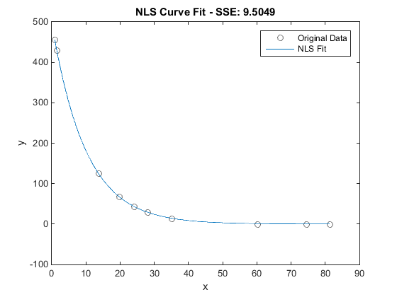
Enabling iteration printing can be quite useful in these problems, as it shows the progression of the solver, as well as the reason for termination. Note this problem has a nasty term (exp(x2*81.3)) which results in IEEE overflow if x2 is chosen too high. lmder however solves this problem without issue.

When you supply both xdata and ydata, you can plot the resulting fit:

Example 4: Weighted Curve Fitting:

From OPTI v2.05 you can now supply fitting weights directly to the OPTI constructor. This allows you to weight each ydata point, signalling its importance in the optimization process. To supply a weighting vector use the weights argument to the OPTI constructor, supplying a vector the same length as ydata.

Note the weighting vector will be multiplied into problem formulation, thus a weight of 1 is typically regarded as the default weighting.

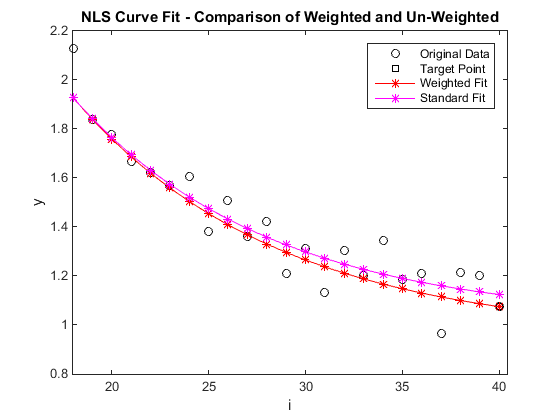
To illustrate, consider the example below where we will heavily weight the last data point. This could be because this point is known to be the most accurate measurement, however for our purposes it is just an example. Any points can be assigned any arbitrary weights.

As shown below the weighted fit has correctly passed through the final data point, as intended. Depending on the range of data within your function you may find larger or smaller weights are required to get the desired fit. Just keep in mind large values can cause numerical problems, so use numbers greater than 1e6 with caution.

Example 5: Supplying Derivatives

So far all examples have automatically utilized Intel's djacobi routine, (implemented in OPTI as mklJac) for approximating both the objective and constraint derivatives via finite differences. While this works OK for small, well behaved problems, real problems you will want to implement your own, exact, derivatives.

Note there are two detailed sections on this topic, 1st Derivatives and 2nd Derivatives, however a small problem will be presented here.

Consider the same problem from Example 1, however this time we will supply exact first derivatives:

Adding first derivative information to OPTI is easy, just tag on the extra arguments:

Note in the NLS case the gradient of the objective is a matrix, where each row is the derivative of a corresponding equation in the objective, and each column is the partial derivative with respect to each decision variable. While strictly speaking this is a Jacobian (as it is partial derivative matrix), OPTI keeps the term Jacobian to refer to the first derivatives of the constraints only, meaning this remains as the gradient. Also note no NLS solver supplied with OPTI currently use sparse first derivatives, so your gradient must be dense.

Example 6: Derivative Free NLS

OPTI does not come with a derivative free NLS solver, but does enable you to solve NLS problems using solvers such as NOMAD or PSWARM by converting it to an NLP. While this not normally advisable (you lose valuable information by doing this conversion), if your problem contains noise or stochastic elements, it may be the best way to obtain a realistic result.

Let's revisit the problem from Example 3:

In the above example, NOMAD finds the same solution as LMDER, as expected. It does however take longer to find this solution, due to extra function evaluations required.

It is also highly recommended to bound your problem (finite upper and lower bounds) when using a global/derivative free solver.

Example 7: Goodness of Fit

From OPTI v2.10 it is now possible to calculate the goodness of fit for a nonlinear least squares solution. OPTI uses RMathLib, a new addition to the toolbox, for calculating the solution statistics and presents it in a way familiar to users of standard statistic software packages.

To illustrate, consider the curve fitting problem from David Himmelblau (Process Analysis by Statistical Methods, 1970):

So far the above construction is the same as what we have seen so far. However a new method, fitStats, allows us to calculate the goodness of the solved fit:

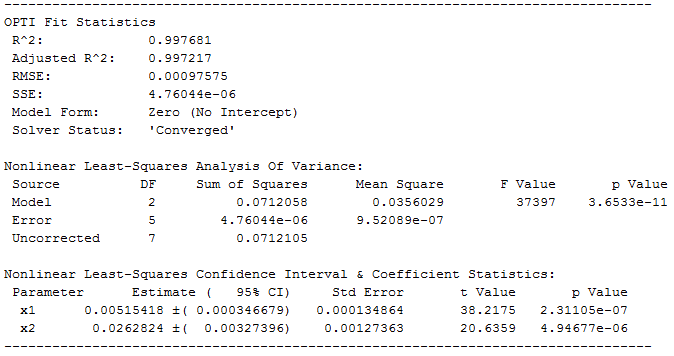
which presents the following information:

If you are unsure what any of these terms mean, consult this page from UCLA. If you are familiar with packages such as SAS, SPSS, or the Statistics Toolbox, then the above should be familiar.

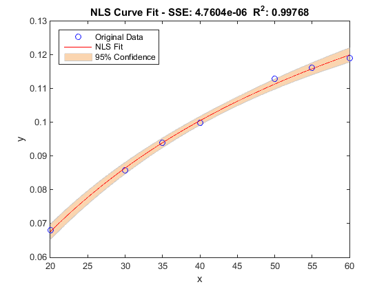
Note fitStats allows the user to specify a customizable confidence interval between 0 and 1 as the second argument, and can return a structure of the printed information for post-analysis. In addition, once fitStats has been called, the confidence interval information is saved in the OPTI object, allowing plot to estimate confidence bounds (functional, simultaneous) of the fit:

Note the confidence bounds will only be plotted if fitStats is called before plot on the OPTI object. Also, the confidence bounds are set by the customizable confidence interval, as described above.