OPTI Toolbox Probs/Quadratically Constrained Quadratic Program (QCQP)

Quadratically Constrained Quadratic Program (QCQP)

Problem Definition

A QCQP has the following form:

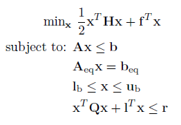
Where H is a n x n sparse matrix (quadratic and bilinear terms) and f is a n x 1 vector (linear terms) containing the quadratic objective function, which is subject to the following constraints:

Linear Inequalities*

A is a m x n sparse matrix, b is a m x 1 vector.

Linear Equalities*

A_eq is a k x n sparse matrix, b_eq is a k x 1 vector.

Decision Variable Bounds

l_b and u_b are n x 1 vectors, where -inf or inf indicate an unbounded lower or upper bound, respectively.

Quadratic Constraints

Q is a n x n sparse matrix, l is a n x 1 vector and r is a 1 x 1 scalar. Multiple quadratic constraints are specified by multiple sets of these three variables. Q must be convex for all solvers other than SCIP.

The goal is to minimize the objective function by selecting a value of x that also satisfies all constraints.

*Your problem description will either use Linear Inequalties and Linear Equalities OR Linear Row Constraints. See the constraint information page.

Note a QCQP is created in a similar way as a QP, so it is recommened you complete reading the QP section before reading the remainder of the section.

Example 1: Small Dense QCQP

Consider the following small QCQP:

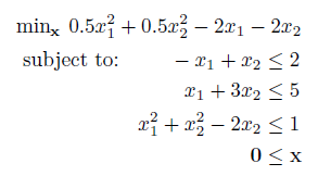
Using the native matrix & vector notation of MATLAB this can be entered as so:

And the problem is solved by passing the problem variables to OPTI, and calling solve on the resulting object:

% Create OPTI Object
Opt = opti('qp',H,f,'ineq',A,b,'lb',lb,'qc',Q,l,r)

% Solve the QCQP problem
[x,fval,exitflag,info] = solve(Opt)

Because the problem contains only two variables, we can use OPTI's built in plot command to view the solution:

plot(Opt)

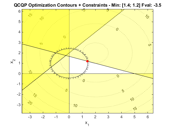
The quadratic constraint is the small black circle near the origin, with the hashing indicating the infeasible side. The optimum must always be inside the quadratic constraint circle. As stated, quadratic constraints must be convex (positive definite) unless you are using a global solver, such as SCIP. For more information on convexity, see the QP page.

Example 2: QCQP with Multiple Quadratic Constraints

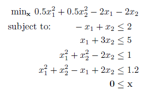
Supplying multiple quadratic constraints requires the user to stack the individual constraints as follows:

Q: A cell array of double matrices, column orientated. Each cell is a constraint Q.
l: A double matrix, where each column is a constraint l vector.
r: A double column vector, where each row is a constraint r scalar.

To illustrate, consider the following example:

% Objective
H = eye(2); %Objective Function (min 0.5x'Hx + f'x)
f = -[2 2]';

% Linear Constraints
A = [-1,1; 1,3]; %Linear Inequality Constraints (Ax <= b)
b = [2;5];
lb = [0;0]; %Bounds on x (lb <= x)

% Quadratic Constraints
Q = {[1 0; 0 1] %Quadratic Inequalities (x'Qx + l'x <= r)
[1 0; 0 1]};
l = [[0;-2] [-1;2]];
r = [1;1.2];

% Create OPTI Object
Opt = opti('qp',H,f,'ineq',A,b,'lb',lb,'qc',Q,l,r)

% Solve the QCQP problem
[x,fval,exitflag,info] = solve(Opt)

% Plot Solution
plot(Opt)

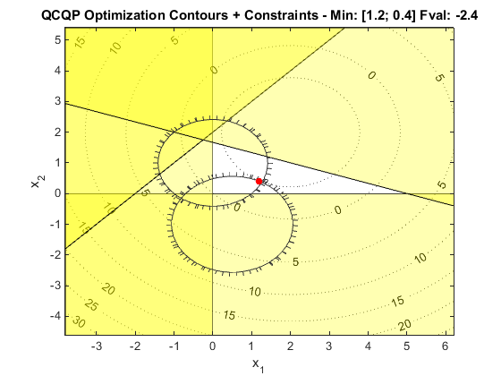
Example 3: QCQP with Multiple Quadratic Constraints [Alternate Setup]

Starting from OPTI v1.79 the user can also supply multiple quadratic constraints using the following cell-based format:

Q: A cell array of double matrices, column orientated. Each cell is a constraint Q.
l: A cell array of double vectors. Each cell is a constraint l vector.
r: A cell array of double scalars. Each cell is a constraint r scalar.

To illustrate, we will revisit the above example:

% Objective
H = eye(2); %Objective Function (min 0.5x'Hx + f'x)
f = -[2 2]';

% Linear Constraints
A = [-1,1; 1,3]; %Linear Inequality Constraints (Ax <= b)
b = [2;5];
lb = [0;0]; %Bounds on x (lb <= x)

% Quadratic Constraints
Q = {[1 0; 0 1] %Quadratic Inequalities (x'Qx + l'x <= r)
[1 0; 0 1]};
l = {[0;-2]; [-1;2]};
r = {1; 1.2};

% Create OPTI Object
Opt = opti('qp',H,f,'ineq',A,b,'lb',lb,'qc',Q,l,r)

% Solve the QCQP problem
[x,fval,exitflag,info] = solve(Opt)

% Plot Solution
plot(Opt)

Example 4: Solving a Positive Semidefinite (PSD) QCQP as a NLP

OPTI will automatically convert (MI)QCQPs to (MI)NLPs if a compatible NLP solver is requested. Currently IPOPT and BONMIN are setup to solve these problems. The OPTI conversion will automatically generate all first and second derivatives, thus the NLP solver can be quite efficient.

To illustrate, consider the following example with a PSD quadratic constraint:

% Objective
H = eye(2); %Objective Function (min 0.5x'Hx + f'x)
f = -[2 2]';

% Linear Constraints
A = [-1,1; 1,3]; %Linear Inequality Constraints (Ax <= b)
b = [2;3.8];
lb = [0;0]; %Bounds on x (lb <= x)
ub = [40;inf];

% Quadratic Constraints
Q = [0 0; 0 10]; %Quadratic Inequalities (x'Qx + l'x <= r)
l = [0;-2];
r = 3

% Set OPTI Options
opts = optiset('solver','ipopt','display','iter');

% Create OPTI Object
Opt = opti('qp',H,f,'ineq',A,b,'bounds',lb,ub,'qc',Q,l,r,'options',opts)

% Solve the QCQP problem [as an NLP]
[x,fval,exitflag,info] = solve(Opt)

% Plot Solution
plot(Opt,3)

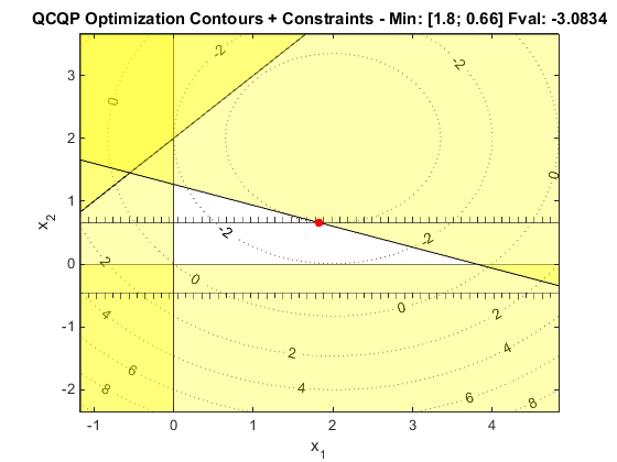
Note solving Positive SemiDefinite (PSD) QPs or QCQPs does not require you to use a NLP solver. However if your problem is indefinite CPLEX will only solve problems with indefinite terms in the objective (i.e. all quadratic constraints must be PSD). For indefinite quadratic constraints then you must use either SCIP (a global solver) or use a NLP solver, as above (noting you may only find a local solution using IPOPT or BONMIN).

Example 5: Quadratic Row Constraints

Starting from OPTI v1.81 you can now supply quadratic constraints in row format, using the following definition:

Note the above format adds extra reasons why the constraint may not be convex. This could be due to:

If qrl = qru, then the quadratic constraint is an equality, and nonlinear equality constraints are non-convex.
If both qrl and qru are finite (i.e. a double-sided constraint), then by definition one side will result in a concave inequality.
As per standard quadratic inequalities, if Q is not positive semi-definite, then the constraint is not convex.

If any of the above conditions are true then you are now solving a non-convex QCQP, which is considerably more difficult to solve! However if you have SCIP installed (a global solver), OPTI will automatically use it to solve your model, as shown below:

% Objective
H = eye(2); %Objective Function (min 0.5x'Hx + f'x)
f = -[2 2]';

% Linear Constraints
A = [-1,1; 1,3]; %Linear Inequality Constraints (Ax <= b)
b = [2;5];
lb = [0;0]; %Bounds on x (lb <= x)

% Quadratic Constraints
Q = {[1 0; 0 1] %Quadratic Constraints (qrl <= x'Qx + l'x <= qru)
[1 0; 0 1]};
l = {[0;-2]; [-2;2]};
qrl = {3; 1}; %QC1 is double sided, QC2 is an equality
qru = {5; 1};

% Create OPTI Object
Opt = opti('qp',H,f,'ineq',A,b,'lb',lb,'qcrow',Q,l,qrl,qru)

% Solve the QCQP problem
[x,fval,exitflag,info] = solve(Opt)

% Plot Solution
plot(Opt)

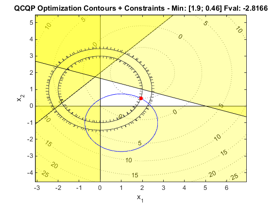
As seen in the above plot, the double-sided quadratic constraint forms a 'donut' shaped feasible region. The quadratic equality is shown in blue, as per the default nonlinear equality constraint colours.

OPTI QCQP Solvers

If you are an academic user and have downloaded the academic version of OPTI a new solver, SCIP, is now included which can solve convex and non-convex QCQPs. Alternatively you can download CPLEX which can solve convex QCQPs to global optimality.

If you do not have these installed OPTI will automatically convert the problem to a MINLP and solve it with IPOPT if no dedicated QCQP solver is available. While not as efficient, all first and second derivative information is passed to IPOPT and it does quite well at solving these problems.

Summary

Solving QCQPs is a complex problem thus long computation times can be expected on large scale problems. Note the 0.5 is dropped from the quadratic constraint definition in OPTI (CPLEX convention).

OPTI Toolbox