Quadratic Program (QP)
Problem Definition
An QP has the following form:
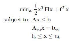
Where H is a n x n sparse matrix (quadratic and bilinear terms) and f is a n x 1 vector (linear terms) containing the quadratic objective function, which is subject to the following constraints:
Linear Inequalities*
A is a m x n sparse matrix, b is a m x 1 vector.
Linear Equalities*
Aeq is a k x n sparse matrix, beq is a k x 1 vector.
Decision Variable Bounds
lb and ub are n x 1 vectors, where -inf or inf indicate an unbounded lower or upper bound, respectively.
The goal is to minimize the objective function by selecting a value of x that also satisfies all constraints.
*Your problem description will either use Linear Inequalties and Linear Equalities OR Linear Row Constraints. See the constraint information page.
Note a QP is created in a similar way as an LP, so it is recommened you complete reading the LP section before reading the remainder of the section.
Example 1: Small Dense QP
Consider the following small QP:
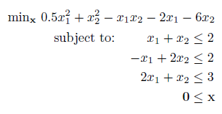
Using the native matrix & vector notation of MATLAB this can be entered as so:
H = [1 -1; -1 2]; %Objective Function (min 0.5x'Hx + f'x)
f = -[2 6]';
% Constraints
A = [1,1; -1,2; 2, 1]; %Linear Inequality Constraints (Ax <= b)
b = [2;2;3];
lb = [0;0]; %Bounds on x (lb <= x)
And the problem is solved by passing the problem variables to OPTI, and calling solve on the resulting object:
Opt = opti('qp',H,f,'ineq',A,b,'lb',lb)
% Solve the QP problem
[x,fval,exitflag,info] = solve(Opt)
Because the problem contains only two variables, we can use OPTI's built in plot command to view the solution:
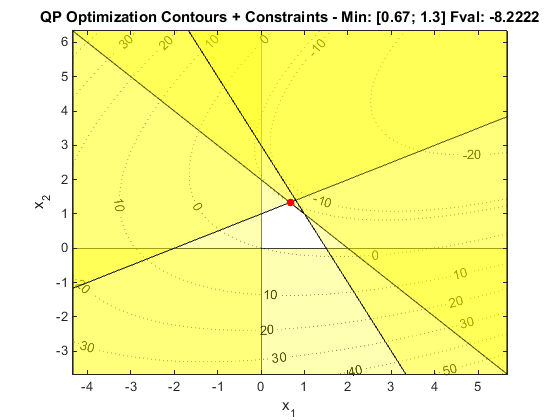
You can see that in contrast to a linear objective, the grey dashed lines (objective contours) are now curves of a quadratic function, rather than straight lines.
Example 2: Sparse QP
As with LPs all QP solvers expect a sparse representation of the constraints, as well as the H matrix. This allows large problems to be solved much more efficiently.
To illustrate, load a QP generated from a Model Predictive Control (MPC) problem supplied as a .QPS problem with OPTI and lets examine the A matrix:
prob = coinRead('MPCqp1.qps')
% Examine A matrix
spy(prob.A)

Note this triangular form is typical of MPC problems, and allows an efficient sparse solver to solve it faster.
To solve this problem, pass the loaded problem structure to the OPTI constructor:
Opt = opti(prob)
% Solve the resulting model
[x,fval] = solve(Opt)
Example 3: (Semi) Positive / Negative Definite QPs
A requirement of most QP solvers is that the H matrix (problem Hessian) must be positive definite. A quick way to check this is to examine the eigenvalues of H (assuming it is symmetric):
If all eigenvalues are positive (and greater than zero), then the matrix is positive definite. The reason this is important is due to convexity. A positive definite QP in two dimensions looks like a bowl:
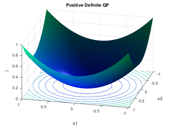
As you can see the above problem has a clear, global optimum at the bottom of the bowl. This concept applies equally to higher dimensions as well.
A negative definite QP (all eigenvalues are negative) is the opposite, a concave hill:
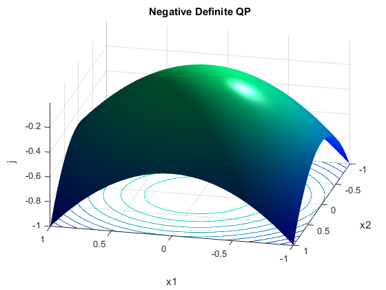
If negated (-H), this problem will be positive definite and we can solve it OK as well. However there are a couple of important variations. Positive semi-definite infers all eigenvalues are greater or equal to zero:
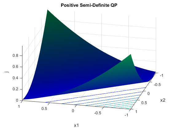
A semidefinite problem looks much more like a valley. However the problem is ill-conditioned when treated as a QP. Try solving the unconstrained minimum and you may see the H matrix is close to singular:
While you can solve semidefinite problems (both positive and negative), using a QP solver is inefficient and is unlikely to return a result.
The final type is the indefinite H, where some eigenvalues are positive and some are negative. This results in a saddle point:
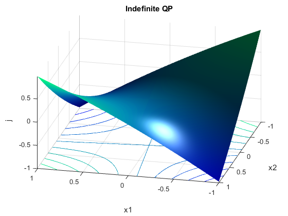
While this problem is well conditioned (unlike the semi-definite one above), the QP solver may not find the global optimum. Consider the following indefinite QP example:

H = [0 -2; -2 0]; %Objective Function (min 1/2x'Hx + f'x)
f = [0 0]';
lb = [-0.5;-0.5]; %Bounds on x (lb <= x <= ub)
ub = [1;1];
% Options
opts = optiset('solver','clp');
% Create OPTI Object
Opt = opti('qp',H,f,'bounds',lb,ub,'options',opts)
% Solve the Indefinite QP
[x,f] = solve(Opt)
As can be seen by plotting the problem:
We have failed to solve the problem at all, even though the solver reports success! (note newer solver versions may actually find the correct solution by chance):
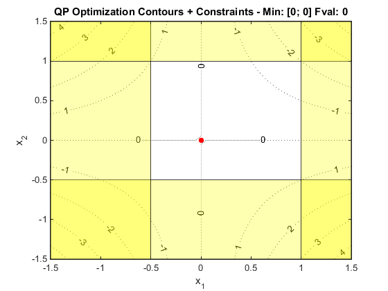
Most QP solvers do not currently allow an initial point to be chosen, thus this is best solution achievable given the problem definition and the solver chosen. The solution - keep your QPs positive definite! If you can't, pose your problem as a GNLP and try a global solver (very inefficient however). If you have the academic version of OPTI you can also use SCIP to solve non-convex QPs to global optimality, or try CPLEX to return a first-order optimal solution (from OPTI v1.79).
Summary
Solving QPs is not too dissimilar to solve LPs, and such you can expect good performance for large problems. Note many solvers expect a triangular form of H, however it varies between upper, lower, and symmetric, depending on the solver. Therefore I suggest you keep your H matrix symmetric, and let OPTI process it.