Semidefinite Program (SDP)
From OPTI v1.80 you can now pose and solve semidefinite problems in OPTI.
Problem Definition
A SDP has the following form (noting OPTI uses the SDPA Standard Primal Form):
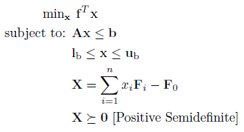
Where f is a n x 1 vector containing the linear objective function, which is subject to the following constraints:
Linear Inequalities
A is a m x n sparse matrix, b is a m x 1 vector.
Decision Variable Bounds
lb and ub are n x 1 vectors, where -inf or inf indicate an unbounded lower or upper bound, respectively.
Semidefinite Constraints
Each Fi is a k x k sparse matrix, and there are (n + 1) F matrices. Multiple semidefinite constraints are specified by multiple sets of these matrices. All F matrices must be symmetric for all solvers.
The goal is to minimize the objective function by selecting the n elements in the vector x that also satisfy all constraints.
Note a SDP is created in a similar way as a LP, so it is recommended you complete reading the LP section before reading the remainder of this section.
Example 1: Single Variable SDP
Consider the following small SDP:
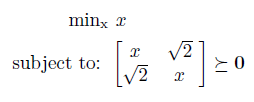
The optimization problem is to find the smallest value of x such that the matrix remains positive semidefinite (all eigenvalues are >= 0). This is known as a Linear Matrix Inequality (LMI). Note that each F is a 2x2 matrix, however there is only one decision variable. In Semidefinite Problems there is no restriction on the size of the LMI matrices, however there must be a matrix for each decision variable + one for the constant term.
To aid showing how this is entered into MATLAB, consider the expanded equation below:

where with reference to the problem definition at the top, we can see how we derive each matrix to create the constraint expression. Also observe each scalar decision variable is element-wise multiplied with each matrix. Given this, the problem can be entered into MATLAB as follows:
f = 1;
% Semidefinite Constraint
F0 = -[0 sqrt(2); sqrt(2) 0];
F1 = eye(2);
sdcone = sparse([F0(:) F1(:)]);
Note each F matrix is converted to a column vector and concatenated into a single sparse matrix, in numerical order (F0,F1,..,Fn). The problem is solved by passing the problem variables to OPTI, and calling solve on the resulting object:
Opt = opti('f',f,'sdcone',sdcone)
% Solve the QP problem
[x,fval,exitflag,info] = solve(Opt)
Example 2: Two Variable SDP
Consider another following small SDP, this time with two variables:
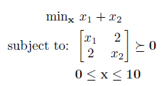
This problem has two variables, thus we need an extra F matrix for x2. However this time we are going to use an alternative nomenclature where C = F0, and A1:n = F1:n , as detailed in the following equation:

This is entered into MATLAB as follows:
f = [1;1];
% Bounds on x (lb <= x <= ub)
lb = [0;0];
ub = [10;10];
% Semidefinite Constraint (using alternative notation)
C = -[0 2; 2 0];
A1 = [1 0; 0 0];
A2 = [0 0; 0 1];
sdcone = sparse([C(:) A1(:) A2(:)]);
% Options
opts = optiset('solver','dsdp','display','iter');
% Create OPTI Object
Opt = opti('f',f,'bounds',lb,ub,'sdcone',sdcone,'options',opts)
% Solve the bounded SDP
[x,f] = solve(Opt)
As can be seen by plotting the problem:
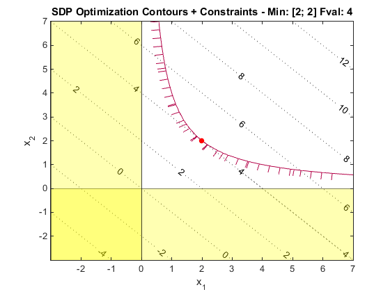
the feasible region is in the upper right of the plot. The red hatched line indicates the boundary of the semidefinite cone constraint.
Example 3: Multiple Semidefinite Constraints
Consider another following small SDP, this time with multiple semidefinite constraints:
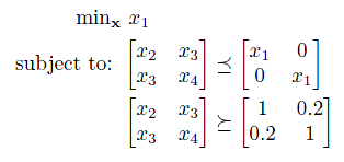
Each semidefinite constraint (i.e. [F0 F1 F2 ..]) is entered as a cell, as follows:
% Objective
f = [1;0;0;0];
% Semidefinite Constraint 1
F0 = zeros(2);
F1 = eye(2);
F2 = -[1 0; 0 0];
F3 = -[0 1; 1 0];
F4 = -[0 0; 0 1];
sdcone{1} = [F0 F1 F2 F3 F4];
% Semidefinite Constraint 2
F0 = [1 0.2; 0.2 1];
F1 = zeros(2);
F2 = [1 0; 0 0];
F3 = [0 1; 1 0];
F4 = [0 0; 0 1];
sdcone{2} = [F0 F1 F2 F3 F4];
% Options
opts = optiset('solver','csdp','display','iter');
% Create OPTI Object
Opt = opti('f',f,'sdcone',sdcone,'options',opts)
% Solve the SDP
[x,f] = solve(Opt)
Also demonstrated in the above example is the ability to supply directly the dense matrices used when constructing the semidefinite constraints. OPTI will recognise the input format and automatically convert it to its internal sparse column representation.
Example 4: Reading Problems in SeDuMi Format
If you are used to creating SDP programs in SeDuMi then you may not want to begin writing new code (or converting existing programs)! Therefore OPTI will also accept linear and semidefinite constraints specified in SeDuMi format:
load sdp_truss1.mat
% Options
opts = optiset('display','iter');
% Create OPTI Object from SeDuMi Args
Opt = opti('sedumi',At,b,c,K,'options',opts)
% Solve the SDP
[x,f] = solve(Opt)
Note if you have SeDuMi installed on your PC the OPTI will automatically use it to solve problems in SeDuMi format. This way you save the conversion between SeDuMi format and OPTI format for storing SDP problems. You are of course able to solve a SeDuMi problem using any other SDP solver as well!
Summary
The above examples show how to create semidefinite problems that OPTI can understand. However constructing semidefinite constraints in MATLAB can be tedious using the methods above! Therefore you may prefer to use YALMIP, another open-source MATLAB toolbox which provides a powerful and easy to use modelling language for semidefinite problems (and many other optimization problems).
If you have problems in SDPA files see the SDPA Reading example for how to load these into OPTI.