System of Nonlinear Equations (SNLE)
Problem Definition
An SNLE has the following form:

Where F is a vector function containing the nonlinear equations.
The goal is to set the function values of all equations to zero by selecting a value of x. This problem is known as root solving, or multivariable root solving when the dimension of x is greater than 1.
Note a SNLE is created in a similar way as a NLS problem. It is recommened you complete reading the NLS section before reading the remainder of the section.
Example 1: 2x2 System
OPTI contains one SNLE solver, HYBRJ from MINPACK. It can be used to solve square systems, where the number of equations equals the number of unknowns, such as in the following system:

To setup this problem, it can be entered as follows (note the API has changed from OPTI v2.05):
nleq = @(x) [ 2*x(1) - x(2) - exp(-x(1));
-x(1) + 2*x(2) - exp(-x(2))];
% Starting Guess
x0 = [-5;5];
And the problem solved by passing the problem variables to OPTI, and calling solve on the resulting object:
Opt = opti('nleq',nleq,'x0',x0)
% Solve the SNLE problem
[x,fval,exitflag,info] = solve(Opt)
However, if you inspect the resulting OPTI object (Opt), you will find that NL2SOL (a NLS solver) has been chosen by OPTI to solve the problem. This is because several NLS solvers have also been setup to solve SNLE problems, by specifying ydata as zeros. As the problems are similar, NLS solvers appear to do quite well at solving these types of problems as well.
As in other examples, you are free to change the solver to override OPTI's choice. To examine all solvers setup to SNLE problems, you can use:
Example 2: Supplying Sparse Derivatives
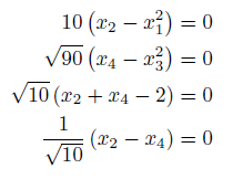
Consider the following 4x4 system of nonlinear equations (modified version of the Wood function):

While we could supply this to OPTI to solve directly, there may be times where using dense first derivatives of our equations can be very memory intensive (i.e. large problems). In these cases it is possible to setup the problem as an NLP in order to leverage sparse derivatives. The below example shows that the problem is entered near identically as above, but when sparse derivatives are supplied, OPTI will automatically convert the problem to an NLP to leverage sparsity.
nleq = @(x) [10*(x(2) - x(1)^2)
sqrt(90)*(x(4) - x(3)^2)
sqrt(10)*(x(2) + x(4) - 2)
(1/sqrt(10))*(x(2) - x(4))];
% Nonlinear Equations Jacobian
nlJac = @(x) sparse([-20*x(1),10,0,0
0,0,-6*10^(1/2)*x(3),3*10^(1/2)
0,10^(1/2),0,10^(1/2)
0,10^(1/2)/10,0,-10^(1/2)/10]);
% Jacobian Sparsity Pattern
nlJacstr = @() sparse([1 1 0 0
0 0 1 1
0 1 0 1
0 1 0 1]);
% Starting Guess
x0 = [-30;-10;-30;-10];
% Sparse SNLE OPTI Problem
Opt = opti('nleq',nleq,'nlJac',nlJac,'nlJacstr',nlJacstr,'x0',x0)
% Solve
[x,fval,exitflag,info] = solve(Opt)
The above code will solve the problem as a NLP which can leverage sparsity, which for larger problems can result in a significant speed-up. Remember you can also supply the Hessian for the NLP for typically even faster convergence. See the example pages on 1st Derivatives and 2nd Derivatives for more information on supplying problem derivatives.