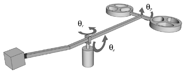
3DOF Helicopter Controller
jMPC Reference: Examples/Documentation Examples/Heli_Example.m
Problem Reference: Åkesson, J., MPCtools 1.0 - Reference Manual, Lund Institute of Technology, 2006
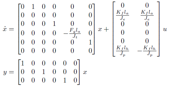
Linear System Model
The continuous time state space equation of the helicopter is as follows:
where we have defined the state vector, x, as:
| x1 | Elevation Angle | [rad] |
| x2 | Elevation Angular Velocity | [rad/s] |
| x3 | Rotation Angle | [rad] |
| x4 | Rotation Angular Velocity | [rad/s] |
| x5 | Pitch Angle | [rad] |
| x6 | Pitch Angular Velocity | [rad/s] |
and the output vector, y, as:
| y1 | Elevation Angle | [rad] |
| y1 | Rotation Angle | [rad] |
| y3 | Pitch Angle | [rad] |
and input, u, as:
| u1 | Motor 1 Voltage | [V] |
| u2 | Motor 2 Voltage | [V] |
Control Objectives
The control objective is to control the Elevation & Rotation angles (y1, y2) to their respective setpoints, by adjusting Motor 1 and 2 Voltages (u1, u2). The Pitch Angle (y3) is constrained but not controlled to a setpoint.
System Constraints
Both Motor Voltages are constrained as:
⚠ $-3\text{V} \le u_{[1-2]} \le 3\text{V}$
Each axis rotation angle is constrained as follows (in radians):
⚠ $-0.6 \le y_1 \le 0.6$
⚠ $-\text{pi} \le y_2 \le \text{pi}$
⚠ $-1 \le y_3 \le 1$
Linear MPC Simulation
Step 1 - Create the Plant
The first step is to implement the model equations above into MATLAB as a jSS object to create the System Plant. For this example we will ignore the linearization biases on the system, however for similar examples with biases see Examples/linear_examples.m. The parameters are first defined, then the model A, B, C & D matrices are created and passed to the jSS constructor:
Je = 0.91; % Moment of inertia about elevation axis
la = 0.66; % Arm length from elevation axis to helicopter body
Kf = 0.5; % Motor Force Constant
Fg = 0.5; % Differential force due to gravity and counter weight
Tg = la*Fg; % Differential torque
Jp = 0.0364; % Moment of inertia about pitch axis
lh = 0.177; % Distance from pitch axis to either motor
Jt = Je; % Moment of inertia about travel axis
%Plant
A = [0 1 0 0 0 0;
0 0 0 0 0 0;
0 0 0 1 0 0;
0 0 0 0 -Fg*la/Jt 0;
0 0 0 0 0 1;
0 0 0 0 0 0];
B = [0 0;
Kf*la/Je Kf*la/Je;
0 0;
0 0;
0 0;
Kf*lh/Jp -Kf*lh/Jp];
C = [1 0 0 0 0 0;
0 0 1 0 0 0;
0 0 0 0 1 0];
D = 0;
%Create jSS Object
Plant = jSS(A,B,C,D)
Step 2 - Discretize the Plant
Object Plant is now a continuous time state space model, but in order to use it with the jMPC Toolbox, it must be first discretized. A suitable sampling time should be chosen based on the plant dynamics, in this case use 0.12 seconds:
Ts = 0.12;
Plant = c2d(Plant,Ts);
Step 3 - Create Controller Model
Now we have a plant to use for simulation, we also need a controller model for the internal calculation of the controller. The plant does not have to be the same as the controller model, and in real life will not be. However for ease of this simulation, we will define the plant & model to be the same:
Step 4 - Setup MPC Specifications
Following the specifications from this example's reference, enter the following MPC specifications:
Np = 30; %Prediction Horizon
Nc = 10; %Control Horizon
%Constraints
con.u = [-3 3 Inf;
-3 3 Inf];
con.y = [-0.6 0.6;
-pi pi;
-1 1];
%Weighting
uwt = [1 1]';
ywt = [10 10 1]';
%Estimator Gain
Kest = dlqe(Model);
Step 5 - Setup Simulation Options
Next we must setup the simulation environment for our controller:
T = 300;
%Setpoint
setp = zeros(T,3);
setp(:,1) = 0.3;
setp(125:250,1) = -0.3;
setp(:,2) = 2;
setp(200:end,2) = 0;
%Initial values
Plant.x0 = [0 0 0 0 0 0]';
Model.x0 = [0 0 0 0 0 0]';
Step 6 - MPC Options
For advanced settings of the MPC controller or simulation you can use the jMPCset function to create the required options structure. For this example we just wish to set the plot titles and axis:
opts = jMPCset('InputNames',{'Motor 1 Voltage','Motor 2 Voltage'},...
'InputUnits',{'V','V'},...
'OutputNames',{'Elevation Angle','Rotation Angle','Pitch Angle'},...
'OutputUnits',{'rad','rad','rad'});
Step 7 - Build the MPC Controller & Simulation Options
Now we have specified all we need to build an MPC controller and Simulation environment, we call the two required constructor functions:
MPC1 = jMPC(Model,Np,Nc,uwt,ywt,con,Kest,opts)
simopts = jSIM(MPC1,Plant,T,setp);
MPC1 is created using the jMPC constructor, where the variables we have declared previously are passed as initialization parameters. simopts is created similarly, except using the jSIM constructor. Both constructors contain appropriate error checking thus the user will be informed of any mistakes when creating either object.
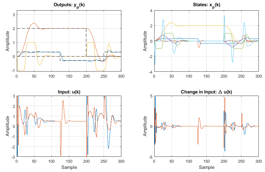
Step 8 - Run the MPC Simulation & Plot Results
With the controller and environment built, we can run the simulation, and plot the results:
simresult = sim(MPC1,simopts)
plot(MPC1,simresult);
The plot produced is shown below:
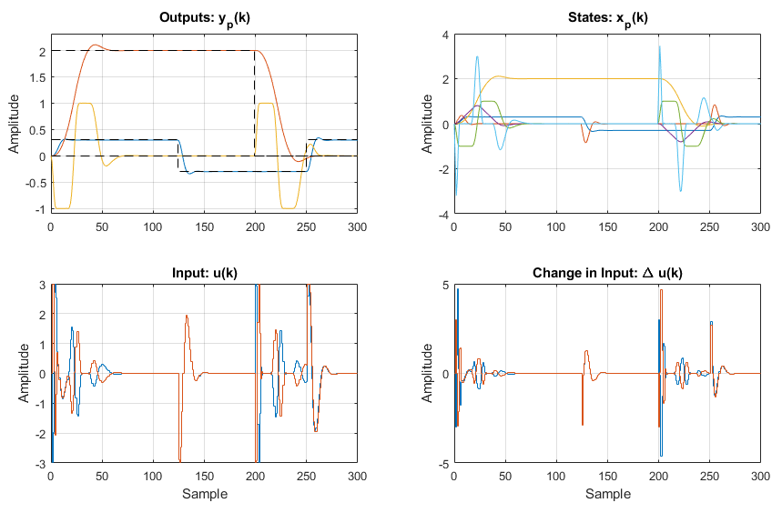
We can also plot a detail plot (using the 'detail' switch) to better view the output responses with respect to the constraints:
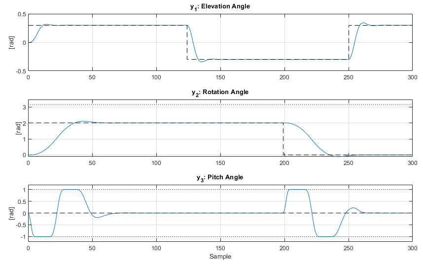
Viewable above is the controlled response with both the elevation angle and rotation angle appearing controlled, with minimal overshoot and fast rise and fall times. Note the pitch angle is constrained as required at ± 1 rad when moving the helicopter around the rotation axis, as was specified.
Linear MPC with Nonlinear Simulation
In order to more accurately verify the controller tuning, we can also create the nonlinear model of the plant, using the non linear differential equations of the helicopter system:
Step 1 - Build Nonlinear ODE Callback Function
As detailed in creating a jNL object, the first step is to write an m-file which contains the above expressions, suitable for use with a MATLAB integrator:
% Nonlinear Helicopter Model
%Assign Parameters
[Je,la,Kf,Fg,Tg,Jp,lh,Jt] = param{:};
xdot(1,1) = x(2);
xdot(2,1) = (Kf*la/Je)*(u(1)+u(2))*cos(x(5))-Tg/Je;
xdot(3,1) = x(4);
xdot(4,1) = -(Fg*la/Jt)*sin(x(5));
xdot(5,1) = x(6);
xdot(6,1) = (Kf*lh/Jp)*(u(1)-u(2));
end
The file, nl_heliUser.m, is saved in a suitable folder on the MATLAB path.
Step 2 - Build the jNL Object
The next step is to build the jNL object, passing the function above as a function handle:
param = {Je,la,Kf,Fg,Tg,Jp,lh,Jt}; %parameter cell array
Plant = jNL(@nl_heliUser,C,param);
Note we have passed the parameters as a cell array, and also retained the linear C output matrix for now. This could also be a function handle to a nonlinear output function.
Step 3 - Linearize the jNL Object
In order to use the nonlinear plant with our linear MPC controller, we must linearize the ODE function and generate the required linear state space model:
u0 = [Tg/(2*Kf*la) Tg/(2*Kf*la)];
Model = linearize(Plant,u0);
In this instance we have chosen the linearize the ODE expression above about the motor voltages of 0.5V. We have not specified a state to linearize about (only an input), such that function will also automatically determine a steady state to linearize about.
Step 4 - Rebuild jSS Object
The model returned from the linearize function is a MATLAB lti object, and can be automatically converted to a jSS object, and then converted to a discrete model:
Model = jSS(Model);
%Discretize model
Model = c2d(Model,Ts);
Step 5 - Rebuild & Re-Simulate the MPC Controller
The last step is to rebuild the MPC controller & simulation environment, and then re run the simulation:
MPC1 = jMPC(Model,Np,Nc,uwt,ywt,con,Kest,opts)
simopts = jSIM(MPC1,Plant,T,setp);
%Re-Simulate & Plot
simresultNL = sim(MPC1,simopts)
plot(MPC1,simresultNL);
The output result is shown below:
As viewable in the plot above, the controlled response of the nonlinear system is quite similar to the linear system, however viewing the plots side by side shows the differences (specifically the nonlinearities):
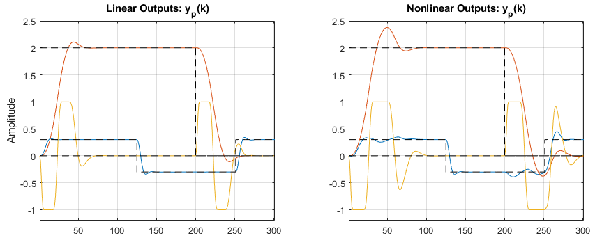
From the nonlinear plot, it is now evident there is significantly more overshoot on the rotation setpoint. This is attributed to the nonlinear equation governing the relationship between the rotation angle, and the pitch angle (sine), which cannot be fully defined a single linearization point. However the control is still reasonable, and would expect to function sufficiently well on a real plant. Note also that further tuning may improve this response, which is left to the reader to implement.