Binary Distillation Column Controller
jMPC Reference: Examples/Documentation Examples/DistillColumn_Example.m
Problem Reference: Hahn, J. and Edgar, T.F., An improved method for nonlinear model reduction using balancing of empirical gramians, Computers and Chemical Engineering (26), 2002
Nonlinear System Model
The continuous time, ordinary differential equations of the column model are as follows:
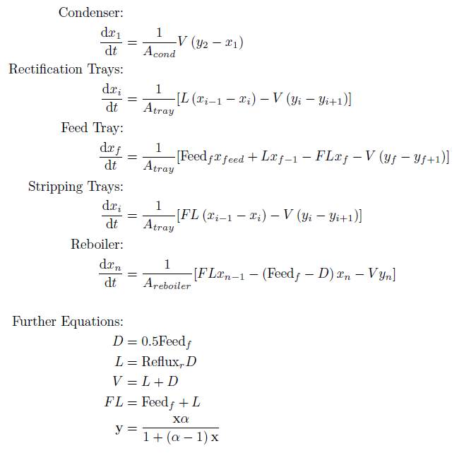
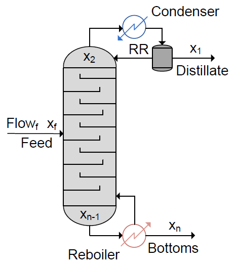
The equations represent a binary distillation column with n trays and a feed tray which can be located at any tray f. The model assumes a constant relative volatility to determine vapour flows.
We have defined the state vector, x, as:
| x1 | Reflux Dum Liquid Mole Fraction of A | [Fraction] |
| x2 | Tray 1 Liquid Mole Fraction of A | [Fraction] |
| x(f) | Feed Tray Liquid Mole Fraction of A | [Fraction] |
| x(n-1) | Tray n Liquid Mole Fraction of A | [Fraction] |
| x(n) | Reboiler Liquid Mole Fraction of A | [Fraction] |
and the output vector, y, as:
| y1 | Reflux Drum Liquid Mole Fraction of A | [Fraction] |
| y2 | Feed Tray Liquid Mole Fraction of A | [Fraction] |
| y3 | Reboiler Liquid Mole Fraction of A | [Fraction] |
and input, u, as:
| u1 | Feed Flowrate (Measured Disturbance) | [mol/min] |
| u2 | Feed Mole Fraction of A (Measured Disturbance) | [Fraction] |
| u3 | Reflux Ratio | [Ratio] |
Control Objectives
The control objective is to control the mole fraction of A in the reflux drum by manipulating the reflux ratio. Both the feed mole fraction and flow rate are measured disturbances, and cannot be modified by the controller. The mole fractions on the other trays are not controlled but constrained within sensible limits.
System Constraints
The reflux ratio is constrained as:
⚠ $0 \le u3 \le 10$
And the tray mole fractions are constrained as:
⚠ $0.98 \le y_1 \le 1$
⚠ $0.48 \le y_2 \le 0.52$
⚠ $0 \le y_3 \le 0.1$
Linear MPC with Nonlinear Simulation
Step 1 - Build Nonlinear ODE Callback Function
As detailed in creating a jNL object, the first step is to write an m-file which contains the above expressions, suitable for use with a MATLAB integrator:
% Nonlinear Distillation model
%Assign Parameters
[FT,rVol,aTray,aCond,aReb] = param{:};
xdot = NaN(size(x));
fFeed = u(1); aFeed = u(2); RR = u(3);
% Additional Eqs
D = 0.5*fFeed; % Distillate Flowrate [mol/min]
L = RR*D; % Flowrate of the Liquid in the Rectification Section [mol/min]
V = L+D; % Vapor Flowrate in the Column [mol/min]
FL = fFeed+L; % Flowrate of the Liquid in the Stripping Section [mol/min]
% Determine Vapour Flows + Delta Flows
y = x*rVol./(1+(rVol-1).*x); % Assume constant relative volatility to determine vapour flows
dx = -diff(x); dy = -diff(y); % Difference molar flow rates
%Calculate flowrates on each tray
xdot(1,1) = 1/aCond*V*(y(2)-x(1)); % Reflux Drum
xdot(2:FT-1,1) = (L*dx(1:FT-2) - V*dy(2:FT-1))/aTray; % Top section
xdot(FT,1) = 1/aTray*(fFeed*aFeed+L*x(FT-1)-FL*x(FT)-V*(y(FT)-y(FT+1))); % Feed tray
xdot(FT+1:end-1) = (FL*dx(FT:end-1)-V*dy(FT+1:end))/aTray; % Bottom section
xdot(end) = (FL*x(end-1)-(fFeed-D)*x(end)-V*y(end))/aReb; % Reboiler
end
The file, nl_distil.m, is saved in a suitable folder on the MATLAB path.
Step 2 - Build the jNL Object
The next step is to build the jNL object, passing the function above as a function handle:
nTrays = 32; % Number of Trays
feedTray = 17; % Feed tray location
rVol = 1.6; % Relative Volatility
aTray = 0.25; % Total Molar Holdup on each Tray
aCond = 0.5; % Total Molar Holdup in the Condensor
aReb = 1.0; % Total Molar Holdup in the Reboiler
aFeed = 0.5; % Feed Mole Fraction
%Output Matrix
C = zeros(3,nTrays);
C(1,1) = 1; C(2,feedTray) = 1; C(3,end) = 1;
%Nonlinear Plant
param = {feedTray,rVol,aTray,aCond,aReb,aFeed}; %parameter cell array
Plant = jNL(@nl_distil,C,param);
Note we have passed the parameters as a cell array, and also retained the linear C output matrix for now. This could also be a function handle to a nonlinear output function.
Step 3 - Linearize the jNL Object
In order to use the nonlinear plant with our linear MPC controller, we must linearize the ODE function and generate the required linear state space model:
fFeed = 24/60; % Feed Flowrate [mol/min]
RR = 3; % Reflux Ratio
%Linearize Plant
u0 = [fFeed aFeed RR]';
x0 = []; %unknown operating point
[Model,xop] = linearize(Plant,u0,x0,'ode15s');
Note in this instance we have specified to use ode15s for linearization. As we do not know the states at our linearization point the linearize function will also solve for the steady state using ode15s, if one exists. This will be returned as xop which can be used for initial states later on.
Step 4 - Create Controller Model
Returned from linearize is a MATLAB lti object containing the linearized model of our system. This must be converted to a jSS object, and discretized to be used to build an MPC controller:
Model = jSS(Model);
Ts = 1;
Model = c2d(Model,Ts)
In order to assign the measured disturbances in the model, we use the following method:
Model = SetMeasuredDist(Model,[1 2]); %Provide index of which inputs are mdist
Step 5 - Setup MPC Specifications
The MPC controller is specified as follows:
Np = 25; %Prediction Horizon
Nc = 10; %Control Horizon
%Constraints
con.u = [0 10 1];
con.y = [0.92 1;
0.48 0.52;
0 0.1];
%Weighting
uwt = 1;
ywt = [10 0 0]';
%Estimator Gain
Kest = dlqe(Model);
Step 6 - Setup Simulation Options
Next we must setup the simulation environment for our controller:
T = 200;
%Setpoint (Reflux Drum)
setp = zeros(T,1);
setp(:,1) = xop(1);
setp(10:end,1) = xop(1)+0.02;
%Measured Disturbances
mdist = zeros(T,2); mdist(:,1) = fFeed; mdist(:,2) = aFeed;
mdist(60:end,2) = aFeed+0.01; %Small increase in feed mole fraction
mdist(140:end,1) = fFeed+1; %Small increase in feed flow rate
%Set Initial values at linearization point
Plant.x0 = xop;
Model.x0 = xop;
Step 7 - MPC Options
For advanced settings of the MPC controller we use the jMPCset function to create the required options structure. For this example we wish to set the plot titles and axis, as well as setting the initial control input (at k = 0) to the linearization point:
opts = jMPCset('InitialU',u0,... %Set initial control input at linearization point
'InputNames',{'Feed Flowrate','Feed Mole Fraction','Reflux Ratio'},...
'InputUnits',{'mol/min','Fraction','Ratio'},...
'OutputNames',{'Liquid Mole Fraction in Reflux Drum','Liquid Mole Fraction in Feed Tray',...
'Liquid Mole Fraction in Reboiler'},...
'OutputUnits',{'Fraction','Fraction','Fraction'});
Step 8 - Build the MPC Controller & Simulation Options
Now we have specified all we need to build an MPC controller and Simulation environment, we call the two required constructor functions:
MPC1 = jMPC(Model,Np,Nc,uwt,ywt,con,Kest,opts)
simopts = jSIM(MPC1,Plant,T,setp,[],mdist);
MPC1 is created using the jMPC constructor, where the variables we have declared previously are passed as initialization parameters. simopts is created similarly, except using the jSIM constructor. Both constructors contain appropriate error checking thus the user will be informed of any mistakes when creating either object.
Step 9 - Run the MPC Simulation & Plot Results
With the controller and environment built, we can run the simulation, and plot the results. We use Simulink as the evaluation environment as it runs significantly faster than Matlab for these simulations:
simresult = sim(MPC1,simopts,'Simulink');
plot(MPC1,simresult,'detail');
The plot produced is shown below:
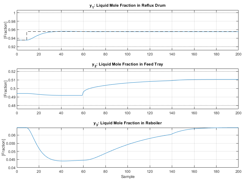
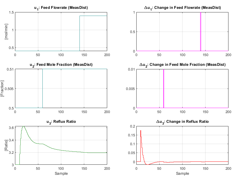
As with the CSTR the linear MPC controller retains good control of the distillation column even when faced with a large nonlinear system with multiple disturbances. An interesting plot to observe is the mole fractions estimated by the model:
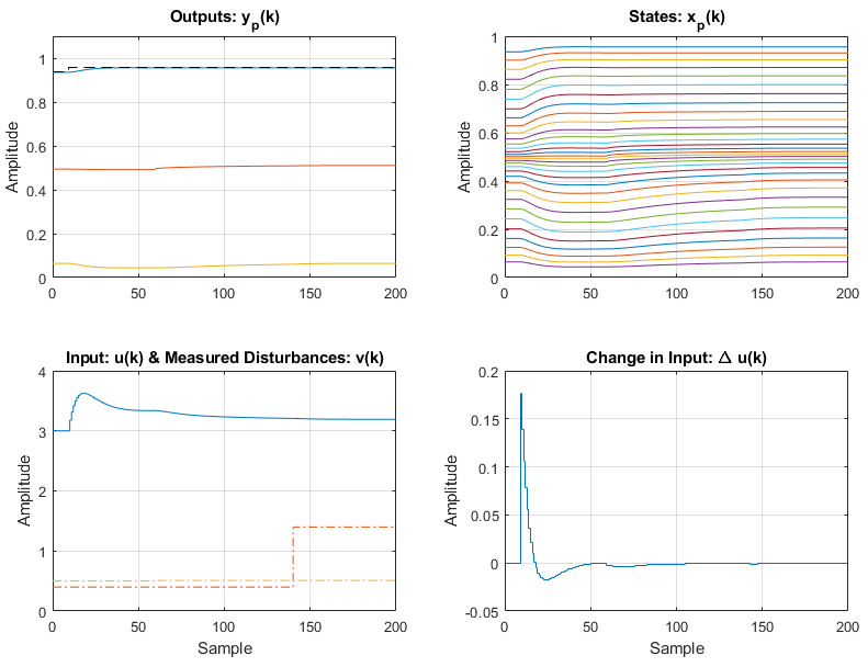
Which is viewable above in the summary figure.