Quad Tank Controller
jMPC Reference: Examples/Documentation Examples/QuadTank_Example.m
Problem References: [1] Åkesson, J., MPCtools 1.0 - Reference Manual, Lund Institute of Technology, 2006; [2] Coupled Water Tanks User Manual, Quanser, 2003
Linear System Model
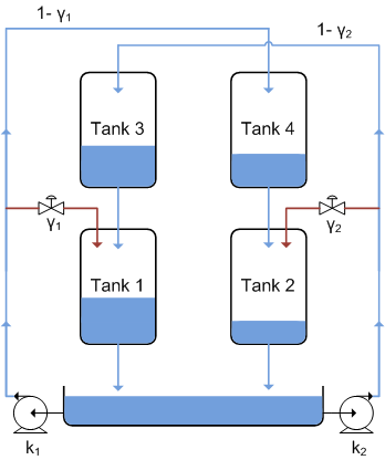
The continuous time state space equation of the 4-tank system is as follows:

where we have defined the state vector, x, as:
| x1 | Tank 1 Level |
| x2 | Tank 2 Level |
| x3 | Tank 3 Level |
| x4 | Tank 4 Level |
and the output vector, y, as:
| y1 | Tank 1 Level | [cm] |
| y2 | Tank 2 Level | [cm] |
| y3 | Tank 3 Level | [cm] |
| y4 | Tank 4 Level | [cm] |
and input, u, as:
| u1 | Pump 1 Voltage | [V] |
| u2 | Pump 2 Voltage | [V] |
Control Objectives
Due to the non-square nature of the system (2 inputs and 4 outputs) we will control two outputs, namely the bottom two tank levels (y1, y2) to a specified setpoint. This will be achieved by controlling the pump voltages via the inputs (u1, u2). The top two tank levels are measured and are also constrained within safe operating limits, but are not directly controlled.
System Constraints
Both Pump Voltages are constrained as:
⚠ $-12\text{V} \le u_{[1-2]} \le 12\text{V}$
The Bottom Two Tank Levels are constrained as:
⚠ $0\text{V} \le y_{[1-2]} \le 25\text{cm}$
And The Top Two Tank Levels are constrained as:
⚠ $0\text{cm} \le y_{[3-4]} \le 10\text{cm}$
Linear MPC Simulation
Step 1 - Create the Plant
The first step is to implement the model equations above into MATLAB as a jSS object to create the System Plant. For this example we will ignore the linearization biases on the system (for simplicity), however for the following example with biases see Examples/linear_examples.m. The parameters are first defined, then the model A, B, C & D matrices are created and passed to the jSS constructor:
%Tank cross sectional area
A1 = 15.5179; A2 = 15.5179; A3 = 15.5179; A4 = 15.5179;
%Outlet cross sectional area
a1 = 0.1781; a2 = 0.1781; a3 = 0.1781; a4 = 0.1781;
%Gravity
g = 981;
%Pump coefficients
k1 = 4.35;
k2 = 4.39;
%Ratio of allocated pump capacity between lower and upper tank
g1 = 0.36;
g2 = 0.36;
%Steady state values
x0 = [15.0751 15.0036 6.2151 6.1003];
u0 = [7 7];
%Constants
T1 = A1/a1*sqrt((2*x0(1)/g));
T2 = A2/a2*sqrt((2*x0(2)/g));
T3 = A3/a3*sqrt((2*x0(3)/g));
T4 = A4/a4*sqrt((2*x0(4)/g));
%Plant
A = [-1/T1 0 A3/(A1*T3) 0;
0 -1/T2 0 A4/(A2*T4);
0 0 -1/T3 0;
0 0 0 -1/T4];
B = [(g1*k1)/A1 0;
0 (g2*k2)/A2;
0 ((1-g2)*k2)/A3;
((1-g1)*k1)/A4 0];
C = eye(4);
D = 0;
%Create jSS Object
Plant = jSS(A,B,C,D)
Step 2 - Discretize the Plant
Object Plant is now a continuous time state space model, but in order to use it with the jMPC Toolbox, it must be first discretized. A suitable sampling time should be chosen based on the plant dynamics, in this case use 3 seconds:
Ts = 3;
Plant = c2d(Plant,Ts);
Step 3 - Create Controller Model
Now we have a plant to use for simulation, we also need a controller model for the internal calculation of the controller. The plant does not have to be the same as the controller model, and in real life will not be. However for ease of this simulation, we will define the plant & model to be the same:
Step 4 - Setup MPC Specifications
Following the specifications from this example's reference, enter the following MPC specifications:
Np = 10; %Prediction Horizon
Nc = 3; %Control Horizon
%Constraints
con.u = [0 12 6;
0 12 6];
con.y = [0 25;
0 25;
0 10;
0 10];
%Weighting
uwt = [8 8]';
ywt = [10 10 0 0]';
%Estimator Gain
Kest = dlqe(Model);
In this case we have chosen a prediction horizon of 10 samples (30 seconds at Ts = 3s) and a control horizon of 3 samples (6 seconds).
Step 5 - Setup Simulation Options
Next we must setup the simulation environment for our controller:
T = 250;
%Setpoint (Bottom Left, Bottom Right)
setp = 15*ones(T,2);
setp(100:end,1:2) = 20;
setp(200:end,2) = 15;
%Initial values
Plant.x0 = [0 0 0 0]';
Model.x0 = [0 0 0 0]';
Step 6 - Build the MPC Controller & Simulation Options
Now we have specified all we need to build an MPC controller and Simulation environment, we call the two required constructor functions:
MPC1 = jMPC(Model,Np,Nc,uwt,ywt,con,Kest)
simopts = jSIM(MPC1,Plant,T,setp);
MPC1 is created using the jMPC constructor, where the variables we have declared previously are passed as initialization parameters. simopts is created similarly, except using the jSIM constructor. Both constructors contain appropriate error checking thus the user will be informed of any mistakes when creating either object.
Step 7 - Run the MPC Simulation & Plot Results
With the controller and environment built, we can run the simulation, and plot the results:
simresult = sim(MPC1,simopts)
plot(MPC1,simresult);
The plot produced is shown below:
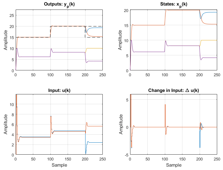
As shown in the top left plot (Outputs) the final step change at k = 200 causes one of the top tanks to hit a constraint, limiting the flow into both bottom tanks. This results in the system being unable to meet the setpoints, which is the desired response (obey constraints first).
Linear MPC Simulation with Unmeasured Disturbances
Step 1 - Add an Unmeasured Input Disturbance & Measurement Noise
This next example will show how to add an unmeasured input (load) disturbance as well as measurement noise to the system. Add the following code in a new cell block:
umdist = zeros(T,2);
umdist(80:end,1) = -1;
noise = randn(T,4)/30;
The variable umdist now contains a 2 column matrix of input disturbance values, which in this case u1 has a 1V bias subtracted from it for samples 80 to 100. The variable noise now contains a 4 column matrix of normal distribution noise, with a mean of 0 and a low power.
Step 2 - Rebuild Simulation
Rebuild the simulation object as follows, this time including the disturbance matrices:
simopts = jSIM(MPC1,Plant,T,setp,umdist,[],noise);
Step 3 - Re-Simulate the MPC Controller
Finally re-simulate the MPC controller with the rebuilt jSIM object:
simresult = sim(MPC1,simopts)
plot(MPC1,simresult);
Which produces the following plot:
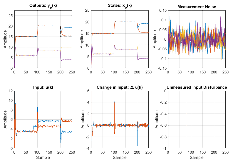
Note the addition of two new axes, which are automatically created when the simulation contains any disturbance. Viewable in the Output axis at sample 80, when the input bias is applied, although the outputs deviate briefly from their setpoints, they quickly return to normal, as the controller compensates with a higher input Voltage, viewable in the Input axis. Also note the measurement noise has a minimal effect on the controlled response, in due partly to the filtering affect of the Kalman Filter and long plant dynamics.
For those interested, re-run the simulation without state estimation and note how the control performance degrades after the input bias is applied, as the plant and model states deviate.