jMPC Toolbox CaseStudies/Servomechanism Controller

Servomechanism Controller

jMPC Reference: Examples/Documentation Examples/Servo_Example.m

Problem Reference: MPC Toolbox v3.2.1, The MathWorks, 2010

Linear System Model

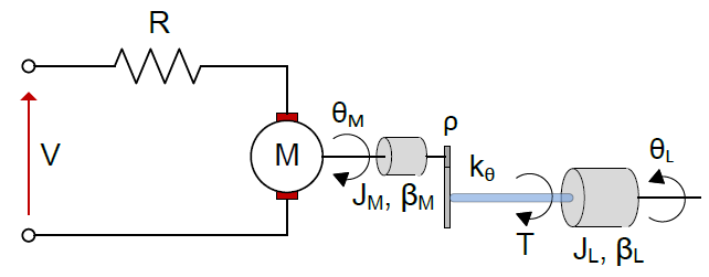
The continuous time state space equation of the servomechanism is as follows:

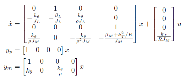
where we have defined the state vector, x, as:

x₁	Load Angle	[rad]
x₂	Load Angular Velocity	[rad/s]
x₃	Motor Angle	[rad]
x₄	Motor Angular Velocity	[rad/s]

and the output vector, y, as:

y₁	Load Angle	[rad]
y₂	Load Torque	[Nm]

and input, u, as:

u₁

Motor Voltage

[V]

Control Objectives

The control objective is to control the Load Angle (y₁) to a desired setpoint, by adjusting the Motor Input Voltage (u₁). We require the Load Angle to settle at the setpoint within around 10 seconds.

System Constraints

The Motor Voltage Constraint is set as:

⚠ $-220\text{V} \le u_1 \le 220\text{V}$

And the Torque Constraint on the shaft is:

⚠ $-78.5\text{Nm} \le y_2 \le 78.5\text{Nm}$

It is important to note in this example that we cannot directly measure the Load Torque, however we must constrain it. This is a perfect example of the power of model based control, where we can use the internal model outputs (y_m) in order to predict unmeasured outputs. The predicted outputs can then be controlled and/or constrained as per a normal output. For this example we will constrain the Load Torque only, and not control it to a setpoint.

Linear MPC Simulation

Step 1 - Create the Plant

The first step is to implement the model equations above into MATLAB as a jSS object to create the system Plant. The parameters are first defined, then the model A, B, C & D matrices are created and passed to the jSS constructor:

%Parameters
k0 = 1280.2; %Torisional Rigidity
kT = 10; %Motor Constant
JM = 0.5; %Motor Inertia
JL = 50*JM; %Load Inertia
p = 20; %Gear Ratio
BM = 0.1; %Motor viscous friction
BL = 25; %Load viscous friction
R = 20; %Armature Resistance

%Plant
A = [0 1 0 0;
-k0/JL -BL/JL k0/(p*JL) 0;
0 0 0 1;
k0/(p*JM) 0 -k0/(p^2*JM) -(BM+kT^2/R)/JM];
B = [0;
0;
0;
kT/(R*JM)];
C = [1 0 0 0]; %Plant Output
Cm = [1 0 0 0; %Model contains unmeasured outputs
k0 0 -k0/p 0];
D = 0;

%Create jSS Object
Plant = jSS(A,B,C,D);

Step 2 - Discretize the Plant

Object Plant is now a continuous time state space model, but in order to use it with the jMPC Toolbox, it must be first discretized. A suitable sampling time should be chosen based on the plant dynamics, in this case use 0.1 seconds:

%Discretize Plant
Ts = 0.1;
Plant = c2d(Plant,Ts);

Step 3 - Create Controller Model

Now we have a plant to use for simulation, we also need a controller model for the internal calculation of the controller. The plant does not have to be the same as the controller model, and in real life will not be. However for ease of this simulation, we will define the plant & model to be the same:

%Create jSS Model
Model = jSS(A,B,Cm,D);
Model = c2d(Model,Ts);

In order to assign the second model output (Torque) as unmeasured, we use the following method:

%Set Unmeasured Outputs in model
Model = SetUnmeasuredOut(Model,2);

Step 4 - Setup MPC Specifications

Following the specifications from this example's reference, enter the following MPC specifications:

%Horizons
Np = 10; %Prediction Horizon
Nc = 2; %Control Horizon

%Constraints
con.u = [-220 220 1e2]; %in1 umin umax delumax
con.y = [-inf inf ; %out1 ymin ymax
-78.5 78.5]; %out2 ymin ymax
%Weighting
uwt = [0.1]';
ywt = [1 0]'; %do not control the second output (Torque)

%Estimator Gain
Kest = dlqe(Model);

In this case we have chosen a prediction horizon of 10 samples (1 second at Ts = 0.1s) and a control horizon of 2 samples (0.2 seconds). The control horizon must always be less than or equal to the prediction horizon, based on the formulation of the MPC problem. The prediction horizon should be chosen based on the dynamics of the system, such that it can predict past any system dead time and sufficient enough for the controller to predict required constraint handling.

The constraints are specified exactly as above, noting a default rate of change of the input Voltage has been chosen as 100V/sample. This variable must be defined if the controller is constrained, however if you are not concerned about the rate of change, you can use a suitably large value, such as done here. Also note the output load angle (y1) is not constrained, such that minimum and maximum are defined as -inf, and inf, which removes that output from constraint handling in the controller.

The weighting is the user's main handle for tuning the controller performance. A larger number represents a larger penalty for that input / output, where inputs are penalized based on a zero input (no plant input), and outputs based on setpoint deviation. Penalizing inputs will discourage the controller from using that input, and penalizing outputs will encourage the controller to move that output to the setpoint faster.

A special function in this toolbox is the ability to set a weight to 0, as done in y2. This tells the MPC constructor this is an uncontrolled output, such that it is not fed-back, and it will not have a setpoint, however you may still place constraints on it, as is done in this example.

The final line creates a discrete time observer using an overloaded version of the MATLAB dlqe function, assuming identity Q & R covariance matrices.

Step 5 - Setup Simulation Options

Next we must setup the simulation environment for our controller:

%Simulation Length
T = 300;

%Setpoint (Load Angle)
setp = ones(T,1);
setp(1:50) = 0;

%Initial values
Plant.x0 = [0 0 0 0]';
Model.x0 = [0 0 0 0]';

The simulation length is always defined in samples, such that in this example it is set to 30 seconds (300 samples x 0.1s). The setpoint must be defined as T samples long, and is a user specified trajectory for the controller to follow throughout the entire simulation. When there are multiple controlled outputs, the setpoint must a matrix, with each column representing a different output.

Finally the initial states of the Plant & Model can be set individually, such that simulations where the controller starts a state mismatch can be tested.

Step 6 - MPC Options

For advanced settings of the MPC controller or simulation you can use the jMPCset function to create the required options structure. For this example we just wish to set the plot titles and axis:

%Set Options
opts = jMPCset('InputNames',{'Motor Voltage'},...
'InputUnits',{'V'},...
'OutputNames',{'Load Angle','Load Torque'},...
'OutputUnits',{'rad','Nm'});

Step 7 - Build the MPC Controller & Simulation Options

Now we have specified all we need to build an MPC controller and Simulation environment, we call the two required constructor functions:

%-- Build MPC & Simulation --%
MPC1 = jMPC(Model,Np,Nc,uwt,ywt,con,Kest,opts)
simopts = jSIM(MPC1,Plant,T,setp);

MPC1 is created using the jMPC constructor, where the variables we have declared previously are passed as initialization parameters. simopts is created similarly, except using the jSIM constructor. Both constructors contain appropriate error checking thus the user will be informed of any mistakes when creating either object.

Step 8 - Run the MPC Simulation & Plot Results

With the controller and environment built, we can run the simulation, and plot the results:

%-- Simulate & Plot Result --%
simresult = sim(MPC1,simopts)
plot(MPC1,simresult);

The sim function will be familiar to most MATLAB users, and is overloaded here for the jMPC Class. Passing the controller and the simulation environment will allow a full MPC simulation to run, with progress indicated by the Progress Bar. In this instance we have specified we wish to run a MATLAB simulation (default), rather than a Simulink or other MPC implementation.

The final command, plot, is once again overloaded for the jMPC Class, and allows us to pass the controller (required for constraint listing), the simulation results, and specify the type of plot we wish to view. In this instance, just a summary will do. The plot produced is shown below:

Viewable in the top left axis (Outputs), the controlled response of the load angle (blue line) is poor, and the value oscillates for some time before we would expect to see it settle.

The next task is to tune the controller such that we achieve a settling period of the load angle within around 10 seconds. Noting the physical constraints on the system, we can see the input Voltage is less than a third of its maximum, such that we can reduce the weight on this input to encourage the controller to use more voltage for a faster response. The Torque is also much lower than the constrained value, such that increasing the voltage shouldn't be a problem.

Step 9 - Re Tune Controller Weights

Decrease the input weight and increase output 1 weight as follows, then rebuild the controller:

%Weighting
uwt = [0.05]';
ywt = [2 0]';

%Rebuild MPC
MPC1 = jMPC(Model,Np,Nc,uwt,ywt,con,Kest,opts)

Step 10 - Re Run MPC Simulation

With the new controller, run the simulation again using the existing simulation environment, and plot the results using the detail switch:

%Re-Simulate & Plot
simresult = sim(MPC1,simopts)
plot(MPC1,simresult,'detail');

The detailed output result is shown below:

Linear Simulink Simulation

Step 1 - Re Run MPC Simulation with Simulink Switch

In order to use the supplied Simulink MPC components, the simplest way to get started is to simply use the 'Simulink' switch:

%Re-Simulate & Plot
simresult = sim(MPC1,simopts,'Simulink')
plot(MPC1,simresult,'detail');

which, all going to plan, will give exactly the same results as the 'Matlab' simulation. This mode populates the supplied jMPC_simulink.mdl Simulink Model with the auto generated MPC components, and calls Simulink to simulate it. The difference here is that the simulation is now running the jMPC Discrete MPC Controller, written in C and supplied as a Simulink block. This code is optimized for general MPC use and thus will run much faster than the Matlab Simulation code. However the m-file algorithm is still useful for those wishing to learn how to create their own MPC implementations (like me), and as such, is still used.

Step 2 - Build a Simulink Model To Test the Controller

Fire up Simulink, and build the following Simulink model using the jMPC Toolbox & Standard Simulink Blocks:

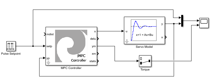
Set the Simulink Solver configuration as follows:

Fixed Step Discrete
0.1s Sampling Time
0 -> 50s run time

Set the Pulse Generator configuration as follows:

Sample based with a sample time of 0.1
Period 400 samples
Pulse width 200 samples
Amplitude of 1
Phase Delay of 0

Set the Selector block as follows:

Input port size of 2
Index as 2

By default the MPC Controller and Plant will have variable names already used in the example above, but you can customize these as you require.

Step 3 - Running the jMPC Simulink Simulation:

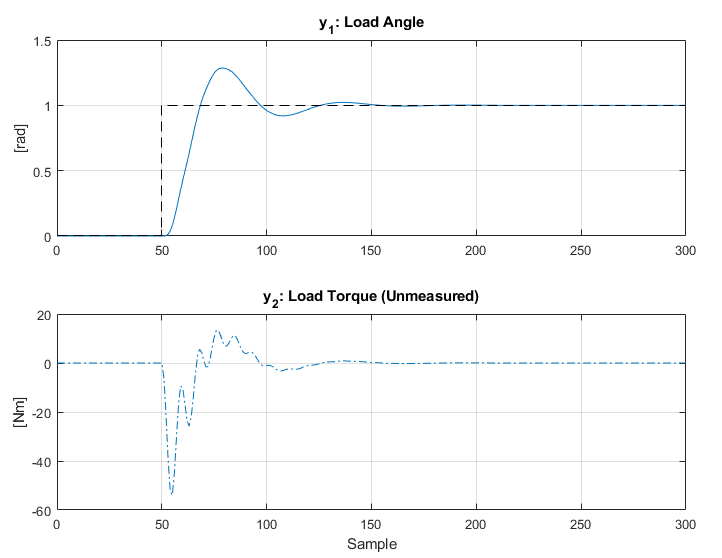
Click Run to generate the following plot in the Scope:

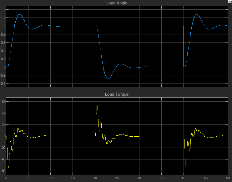
This example shows just how easy it is to create a jMPC MPC Controller in Matlab, import it to Simulink, and then run a Simulink Simulation.

jMPC Toolbox