jMPC Toolbox

Model Predictive Control (MPC) is an Advanced Process Control (APC) technology which is used commonly in the Chemical Engineering and Process Engineering fields. MPC allows control of all plants from Single Input Single Output (SISO) through to Multiple Input Multiple Output (MIMO) and non-square systems (different numbers of inputs and outputs). However its real advantage is the ability to explicitly handle constraints, such that they are included when calculating the optimal control input(s) to the plant. Among other attractive features, this has enabled MPC to be the preferred APC technology for a number of years, and continues to this day.

Several variants of the MPC algorithm exist, including the original Dynamic Matrix Control (DMC), Predicted Functional Control (PFC), Generalized Predictive Control (GPC) as well as nonlinear and linear MPC. However all retain a common functionality; a model of the system is used to predict the future output of the plant so that they controller can predict dead-time, constraint violations, future setpoints and plant dynamics when calculating the next control move. This enables robust control which has proved its use in industry and academia for over 20 years

Linear MPC

The MPC algorithm used within the jMPC Toolbox is a linear implementation, where a linear state space model is used for the system prediction. This enables the controller to formulate the control problem as a Quadratic Program (QP), which when setup correctly results in a convex QP, ensuring an optimal input (global minimum). The fundamental algorithm characteristic is the system prediction and subsequent control move optimization, shown below:

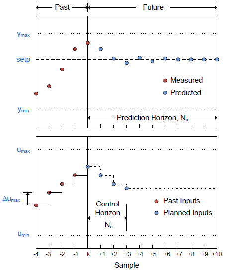
Viewable above is the standard MPC prediction plot, where the top plot shows the predicted plant output for the prediction horizon, and the bottom plot shows the planned control inputs for the control horizon. The linear model which is used to build the controller is used for the plant prediction, viewable as the blue dots. With a good model of your system this prediction can be quite accurate, enabling the control moves to optimally move the system to the setpoint. Also shown in the above plots are the constraints available to MPC including maximum and minimum inputs and outputs, as well maximum rate of change of the input.

The jMPC Controller

The following diagram shows how the jMPC controller is included in a system:

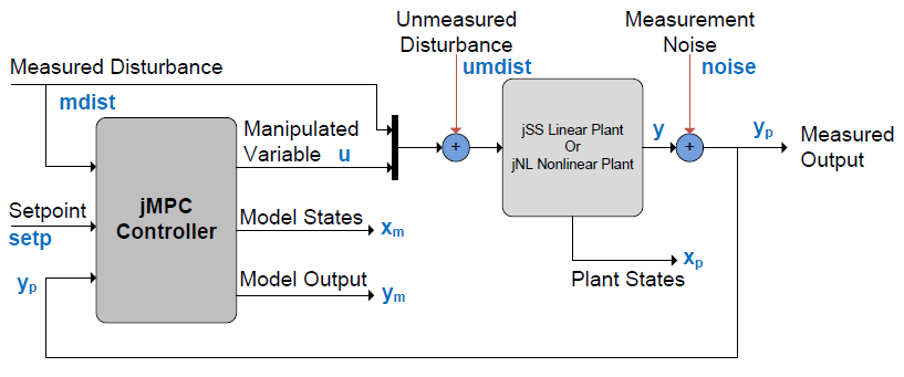
The jMPC controller uses the current setpoint (setp) and measured disturbance (mdist), together with the current plant output measurement (yp) to calculate the optimal control input (u). For simulation purposes you can also add an unmeasured disturbance (umdist) and measurement noise (noise) to the plant to test how the controller responds. For analysis purposes you can also read the model states (xm) and the model output (ym), which can be compared to the plant states (xp) and plant output (yp).

When running a simulation the plant is represented by either a jSS (State Space) linear plant, or a collection of nonlinear (or linear but this is unusual as it should be converted to state space) Ordinary Differential Equations (ODEs) in a jNL plant. This enables you to perform linear and nonlinear simulations using the same jMPC controller, and just changing the plant object.

For more information on the formulation of the MPC problem in jMPC, consult Chapter 3 in my thesis.