jMPC Toolbox

When you have the MATLAB Control Systems Toolbox® installed, this tool can also load lti models for use within MPC simulation. This is the intended purpose of this software, however jSS objects are also provided for use without the Control Systems Toolbox.

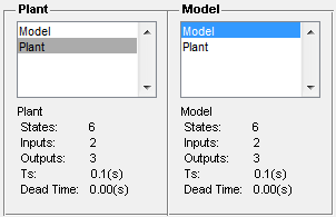
Any MATLAB lti model can be loaded into the GUI, including transfer function (tf), state space (ss), and zero-pole-gain (zpk) models. All of these will appear in the plant & model lists automatically.

Continuous Models

As the underlying Model Predictive Controller is discrete, all models used will be converted to discrete. If Auto Calculate Ts is selected, then the routine described will calculate a suitable sampling rate, and the model will be discretized using the Control Systems Toolbox function, c2d. If Auto Calculate Ts is not selected, then the sampling period entered in the Controller Sampling Period edit box will be used by c2d.

Discrete Models

When Auto Calculate Ts is selected, the Model's sampling period will be used as the Controller Sampling Period. If this option is not selected, and the Plant or Model's sampling time is not the same as the value in the Controller Sampling Period edit box, then it will be re-sampled using the Control Systems Toolbox function, d2d. The same applies if the Plant & Model sampling periods are different.

Problems can occur using d2d on Models which have already been approximated using delay2z. This is due to multiple poles at the origin, which is the effective dead time. In order to avoid this, make sure you either supply discrete models with dead time at the correct sampling rate, or try reselecting the model after changing Ts.

Models with Dead Time

As the original jMPC class does not handle dead time naturally, models supplied with dead time handled differently from those above. The Control Systems Toolbox function, delay2z, is used to convert all dead time into leading zeros in the dynamics, which effectively adds dead time at integer multiples of the sampling time. For continuous models, they are first discretized as above, before this function is applied. This avoids using an approximation such as the function pade. The downside to this method is greater computational load, especially as the dead time increases beyond 10 sampling instants, as the state space matrices are increased in size.

Note the supplied Model object class, jSS, does not have a field for dead time, thus only lti models can be used for dead time simulations.