Graphical User Interface Overview
The function of each of the GUI components is described below.
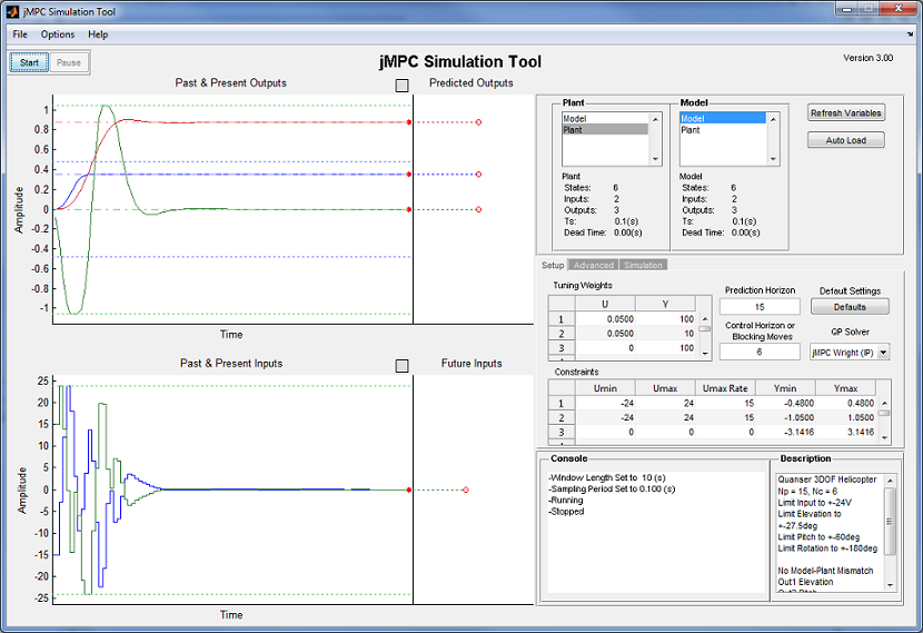
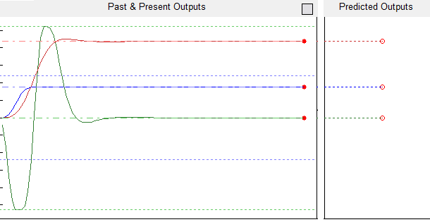
Past & Present Windows
These windows display the current and past data measured by the process. The top window displays the process outputs, while the bottom window displays the process inputs. Using a custom Scrolling Object, these plots scroll as the data is received, allowing only the most recent data to be viewed.
The window size is customizable through the advanced tab.
There are typically 3 lines plotted for each output; the output line itself (solid), the desired setpoint (dash-dot), and the constraints (dotted). For the input the same rules apply but without the setpoint.
Prediction Windows
One of the main advantages of MPC is the predictive component. This window allows you to view in real time the actual predicted response, as calculated using the supplied Model. The upper window is the predicted process output, while the lower window is calculated future input sequence, of which only the first is applied to the plant.
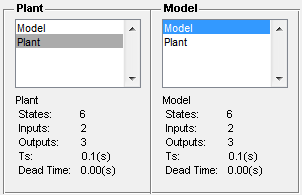
Plant & Model Selection
When running an MPC simulation you must artificially select a Plant to act as the real process. In real life the plant is the real continuous process, and is sampled discretely by the controller. In this software, you load the Plant & Model separately, where the Model is used by the controller exclusively, and the plant for simulation purposes exclusively.
The two lists will only display jSS and lti (ss, zpk, tf) objects, as these are the only compatible models. These models are sourced from the base workspace. If you have added new models to the workspace and wish for these lists to be updated, click "Refresh Variables" to perform a new search of the workspace.
By default this software will automatically select models called "Plant" & "Model" for each list, if they exist.
Tabs
Due to space constraints, 3 tabs have been implemented on the GUI using the user generated function tabpanel. Note that the supplied tabpanel function is covered by a BSD license.
Each of the tabs are described below:
Setup Tab
This is the main Tab used for setting up the MPC controller. It has the following elements:
- Prediction Horizon
- Length of the prediction of the model output
- Control Horizon or Blocking Moves
- Control Horizon (scalar) -> Length of samples calculated as the future input sequence (or)
- Blocking Moves (vector) -> Vector of samples calculated as blocking moves (i.e. [4 2 2 2])
- Tuning Weights
- These are used by the MPC Quadratic Program cost function.
- Placing a higher number will increase the penalty cost as this variable deviates from the setpoint, or for using that input.
- Weights are squared in calculation.
- Constraints
- The fundamental advantage of MPC is the ability to add constraints on the process.
- This software allows constraints on the min and max input, max input change and the min and max output.
- Note all input constraints are hard constraints.
- QP Solver
- In order to compare implementations, 5 QP solvers are available for use, including Matlab's built in
quadprog(provided the Optimization Toolbox is installed).
- In order to compare implementations, 5 QP solvers are available for use, including Matlab's built in
- Default
- When starting out, this button automatically fills in default values within all settings, allowing almost single click simulation.
- Note these values are dependent on the Model size only, and no heuristics are used in choosing values.
Advanced Tab
These settings, although listed as advanced, will likely be required to be used in order to gain the desired result. The properties are:
- State Estimation
- To account for Model - Plant mismatch and the affect of noise, state estimation allows the plant states to be estimated.
- The estimate is applied to the model states via a gain matrix, of which one is designed using a gain supplied by the slider bar.
- Controller Sampling Period
- This is a highly important period, and must be chosen with consideration. Models with different sampling periods will be re sampled at this frequency.
- Window Length
- Determines the length of time visible on the past & present windows.
- Note a maximum of 100 samples can be displayed in the window, so choose a window length appropriate to the sample time.
- Soft Output Constraints
- Enables a penalty weighting on the output constraints such that breaking the output constraints (due to for example a disturbance) does not render the QP problem infeasible. Defaults to a small penalty term for example use.
- Initial Setpoints
- To prevent initial instability, or to start with a transient, use this table to set the setpoints at sample k = 0.
- Simulation Speed
- To slow down the execution of the simulation you can enable 'Slow Mode' which will run the simulation at approximately 1/2 speed.
Simulation Tab
This tab is automatically selected when Start is pushed, and allows editing of Real Time Setpoints & Disturbances. The properties are:
- Setpoint
- With the correct output selected, you can modify in real time the setpoint value. Note due to this being a real time implementation, setpoint look ahead cannot be used.
- The setpoint ranges from -10 to 10, thus the system must be normalised for values outside this range.
- Measurement Noise
- This adds a normally distributed noise signal to the selected output. The power of the noise is selected by the slider.
- Note the slider value ranges from -5 to 5, and the value displayed and added to the output is 10 to the power of this value.
- Load Disturbance
- This adds a bias term to the selected input. The value of the bias is selected by the slider.
- Note the slider ranges from -5 to 5.
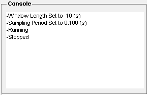
Console
To prevent the need for the user to check run time messages being displayed in the command window, a console is used within the GUI to alert the user of actions being undertaken on their behalf. It is important to identify each message, as they will often lead to undesirable results if ignored.
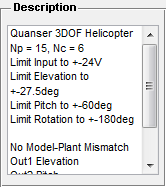
Description
This control is optional, and provided simply for adding a description to the current setup. This description is saved as part of the GUI object, and thus can help you identify objects at a later stage. Note this only updates when an example is loaded, or the user enters information.
Buttons
- Start / Stop
- Simply starts or stops the simulation. Note the same button changes function depending on whether the simulation is running or stopped.
- Pause
- Pause execution of the simulation, without losing the current data
- Refresh Variables
- When you add new or change models / objects to the workspace, this button allows the GUI to rescan the base workspace for changes. Any new models or changes will be identified and populated within the respective lists.
- Auto Load
- This button is covered in detail in the Auto Setup section.