plot
Plot the results from a jMPC Simulation.
Syntax
plot(jMPCobj,jSIMobj)
plot(jMPCobj,jSIMobj,mode)
plot(jMPCobj,jSIMobj,plot_model)
Description
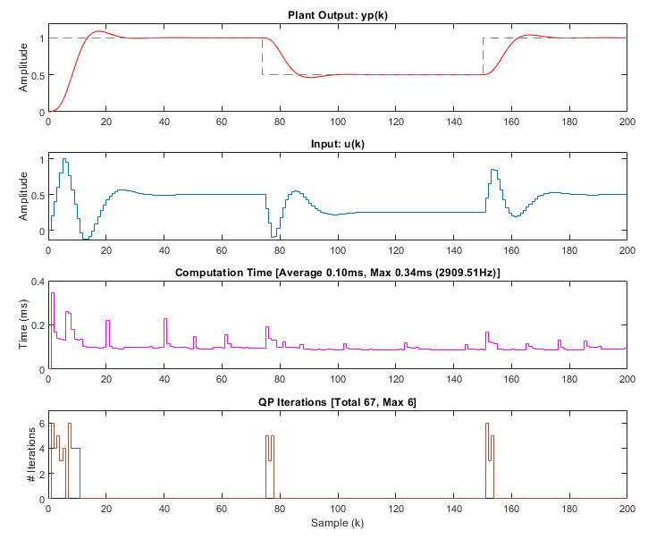
plot(jMPCobj,jSIMobj) takes the simulation results stored in the jSIMobj, together with the controller sizes & setup in the jMPCobj, and generates a summary plot, shown in the plot examples below.
plot(jMPCobj,jSIMobj,mode) allows the user to specify the plot mode from the following:
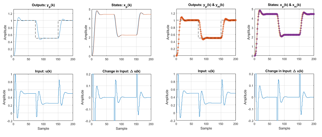
'summary' | A single figure overview of the simulation |
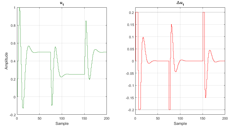
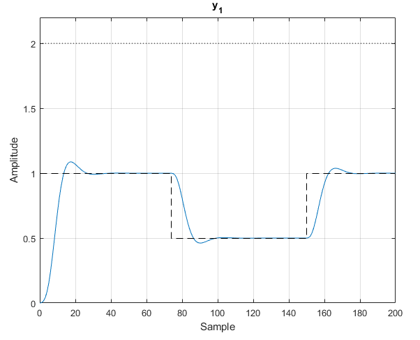
'detail' | A summary figure (above) with 1 figure detailing the outputs, and 1 figure detailing the inputs. Horizontal lines indicating constraints will be automatically drawn if they fall within a dynamic tolerance of the response. If names have been added to the inputs and outputs these will also be drawn on these plots. |
'timing' | A timing summary plot. |
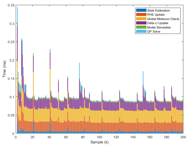
'timingbreakdown' | A timing breakdown plot. Only available for MATLAB simulations. |
plot(jMPCobj,jSIMobj,mode,plot_model) specifies whether the MPC model states and outputs are plotted on top of the plant states and outputs. 1 enables this feature and 0 (default) disables this feature. Useful for comparing simulations when the Model and Plant are different (e.g. one is nonlinear).
Example Plots
All plots below are generated from the linear MPC example - Oscillatory SISO Example, in the Examples folder.
Summary [Left], Summary with Model Output & States [Right]
Detail
Timing
Timing Breakdown
Note this plot type is only compatible with MATLAB jMPC Simulations (not MEX or Simulink).